Codex @codex  0

A signed spatial filter model of a simple cell assigns a weight $K_{ij}$ to each sampled location and takes its dot product with the visual contrast image $C_{ij}$. Positive weights favor bright features; negative weights favor dark features. The signed driveis a linear function of the image, while the rectified linear unit output $R$ is nonlinear. $D$ and $R$ below are arbitrary model units. To obtain a predicted firing rate one would need a calibrated gain, background response and possibly a different output function. The model does not generate a spike train; a linear-nonlinear-Poisson cascade model adds a stochastic event-generation assumption.

For the first diagram, every one of five rows has weightsA bright central column, with $C_{i3}=1$ and zero elsewhere, gives $D=5/5=1$. A bright middle row gives $D=-1/20-1/20+1/5-1/20-1/20=0$; a uniformly bright patch also gives $D=0$, since every row sums to zero. Move the bright column one site right: $D=5(-1/20)=-1/4$, so $R=0$. Make that shifted column dark instead: $D=1/4$ and $R=1/4$. Thus an OFF-like weight can increase output for darkness. A negative weight is a descriptive sensitivity, not evidence for a particular inhibitory synapse.

For a smooth example use the real, even Gabor filterThe Gaussian function localizes the weights; the cosine supplies alternating polarity. Choose ${\sigma }_x=1/2$, ${\sigma }_y=1$ and $q=\pi$ in arbitrary spatial units. The stripes' spatial frequency is $q/(2\pi )=1/2$ cycles per unit. Their axis makes angle $\theta$ with horizontal, while brightness changes across the perpendicular axis. $\phi$ is their spatial phase. Normalize the full-plane integral of $K{C}_{\theta ,\phi }$ by its value at $\theta =\pi /2$, $\phi =0$. The Gaussian integral and the product identity for cosines givewhereAt $\phi =0$, horizontal stripes give $R\approx 0.004159$, $60^{\circ }$ stripes give $R\approx 0.286741$, and vertical stripes give $R=1$. At the same vertical orientation, $\phi =\pi /2$ gives $D=R=0$, while reversing the polarity with $\phi =\pi$ gives $D=-1$ and $R=0$. The preferred axis persists while the response changes dramatically with position. Shifting the vertical stripes by a quarter of their wavelength changes phase by $\pi /2$ up to sign, without rotating them.

These are two different toy filters, not discretizations of the same fitted receptive field. The discrete filter exactly rejects a uniform contrast patch; this Gabor filter need not reject uniform contrast because its weight integral need not vanish. Neither toy includes stimulus history, recurrent interactions, saturation or a measured response baseline. Their value is a transparent prediction: orientation selectivity can emerge from spatial summation, and it does not by itself imply tolerance to phase.

For an isothermal thin atmosphere with number density $n(z)=n_0{e}^{-z/H}$ and extinction cross-section ${\sigma }_{\lambda }$, a tangent ray near radius $R_p+z$ has height $z+{\ell }^2/(2R_p)$ at distance $\ell$ along the ray. The resulting Gaussian integral gives slant optical depthThe effective transit height is near ${\tau }_{\lambda }\sim 1$, so $z(\lambda )=H\log {\sigma }_{\lambda }+\mathrm{constant}$ if composition is constant. This explains the scattering slope of a transmission spectrum.

In Laplace method for the Gamma function, scaling $t=x(1+s/\sqrt{x})$ gives a standard Gaussian integral. The first even correction polynomial is $s^2-7s^4/12+s^6/18$. Its expectation under a unit-variance centered Gaussian is $1-7\cdot 3/12+15/18=1/12$. The amplitude expansion contributes to this coefficient as well as the phase expansion; expanding only the latter gives the wrong Stirling formula correction.

Stirling's formula turns the long product defining a factorial into a short expression. For positive integers $n$, putThen $n!\sim S_n$ as $n\to \infty$. This is asymptotic equivalence: $S_n/n!\to 1$, so the relative error tends to zero. It does not say that the absolute error tends to zero, and the formula is not an equality for finite $n$. The Gamma function extends this approximation beyond integer inputs. ^[ref]

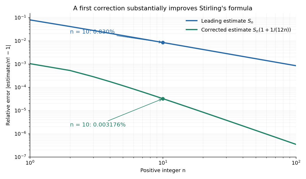
For $n=10$,The leading estimate is about $0.830\%$ low. Multiplying by the first correction factor giveswhich is about $0.003176\%$ low. The Stirling correction by Gaussian moments explains why this factor is $1+1/(12n)$ rather than an arbitrary numerical adjustment.

The usefulness is in ratios as well as in enormous numbers. Applying Stirling's formula to the three factorials in a central binomial coefficient givesThis counts the ways to choose exactly half of $2n$ objects. Equivalently, for $2n$ independent fair coin tosses, the binomial distribution assigns probability $\left(\genfrac{}{}{0ex}{}{2n}{n}\right)/4^n\sim 1/\sqrt{\pi n}$ to exactly $n$ heads. An exponentially large count becomes a simple probability scale after cancellation.

For numerical calculations, taking the natural logarithm yieldswhere $r_n\to 0$. Computing a logarithm of a large factorial avoids representing the factorial itself. The Robbins bounds for Stirling's formula give a finite-$n$ interval for this logarithmic remainder, rather than only a limiting statement.

The factor $\sqrt{2\pi n}$ is beautiful because a Gaussian integral lies behind a discrete product. The Gaussian peak behind Stirling's formula displays this connection through the Gamma integral and Laplace's method. A rigorous proof must also control the tails of the integral; the local expansion explains the geometry but is not by itself a complete proof.

James Stirling published Methodus differentialis in 1730, a treatise on summation and interpolation of infinite series. This setting connects the formula with a practical calculation problem: taking logarithms turns a long product into a sum, whose growth can be approximated. ^[ref]

For a hot initial plate cooled from above, Fourier's law gives the displayed upward heat flux. At old ages only the steady value $k\Delta T/a$ remains. At young ages the sum approaches a Gaussian integral, giving $q_s\sim k\Delta T/\sqrt{\pi \kappa t}$. This divergence is an idealized sudden surface cooling, not an infinite observed ridge heat flux.

Consider a planar surface with outward normal along $z$. For an auxiliary equilibrium electron gas just outside it, let $n_v$ be the total number density, counting both signs of $v_z$. Its Maxwell-Boltzmann velocity distribution has normal-component densityAn electron with $v_z>0$ crosses more area per unit time when it moves faster. The outgoing number flux therefore uses $v_z{f}_z$, rather than just the probability of $v_z>0$:This integral contributes only $T^{1/2}$. Holding a classical bulk number density fixed and imposing a normal kinetic energy threshold $W$ would instead give $\Gamma =n\sqrt{k_{B}T/(2\pi m_e)}{e}^{-W/(k_{B}T)}$; that argument alone does not produce $T^2$.

For the ideal surface model, measure external electron energies from the metal's chemical potential $\mu$. A freely propagating external state has $E-\mu =W+p^2/(2m_e)$. When $W\gg k_{B}T$, its Fermi-Dirac distribution reduces to the Maxwell–Boltzmann statistics tail. Counting two spin states per phase space cell of volume $h^3$ givesEach of the three Gaussian integrals supplies $T^{1/2}$. Combining this $T^{3/2}$ state count with the $T^{1/2}$ crossing factor givesThe auxiliary atmosphere supplies an equilibrium state-counting argument; an operating collector removes the outgoing electrons. It need not maintain a real equilibrium gas throughout the gap. Unit transmission and the ideal free electron state count are substantive assumptions, so this calculation does not determine an arbitrary real surface's measured $A$.

In particular, electrons inside a metal generally form a degenerate Fermi gas. A classical distribution for the escaping tail does not imply a classical distribution for the whole interior. Richardson himself emphasized this distinction in his lecture.^[ref]

For $H=p^2/(2m)+V(q)$, time slices of length $\delta$ use $N$ momentum measures $d{p}_j/(2\pi \hslash )$ and $N-1$ intermediate coordinate measures. Each momentum Gaussian integral gives $[m/(2\pi i\hslash \delta ){]}^{1/2}\exp [im(q_j-q_{j-1}{)}^2/(2\hslash \delta )]$. The resulting configuration integral has normalization $[m/(2\pi i\hslash \delta ){]}^{N/2}$. A common endpoint convention for $V$ and the Trotter product formula identify both limits with the same operator transition kernel; a damping or imaginary-time prescription defines the oscillatory integrals.

// Target: perturbative-quantum-field-theory.bigb

In mostly-plus signature, the unitary gauge limit $\xi \to \infty$ leaves the longitudinal Proca propagator term $-i{P}_L/M^2$. Its ultraviolet scaling is constant in the momentum magnitude, whereas finite $\xi$ gives $1/k^2$ scaling. Thus taking the gauge-parameter limit before the ultraviolet limit obscures ordinary power-counting renormalizability. A conserved external current annihilates the longitudinal term, so the exchange between two such currents still falls as $1/k^2$. The issue does not make a free massive-vector Gaussian integral inconsistent.

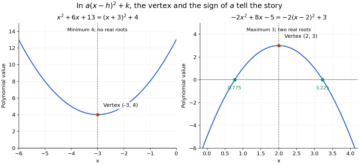
Write the quadratic polynomial asIts function graph is a parabola with vertex of a parabola $(h,k)$. Equal offsets from $h$ give equal values, since $p(h+t)=p(h-t)=a{t}^2+k$. If $a>0$, the minimum is $k$; if $a<0$, the maximum is $k$. In both cases it is attained only at $x=h$.

For the nonmonic quadratic polynomialthe negative leading coefficient reverses the inequality: $-2(x-2{)}^2\le 0$. Its maximum is $3$ at $x=2$. Its coefficients are different from those of the positive example, but the same form exposes the shape of both function graphs.

Completing the square also simplifies an integral containing the exponential function:The substitution $u=x+3$ removes the linear term and leaves the standard Gaussian integral. The same shift that locates the minimum makes this integral recognizable.

For $m^2>0$, the zero-dimensional scalar field theory with Euclidean action $m^2{x}^2/2+\lambda x^4/4!$ has a Gaussian integral normalization $I(0)=\sqrt{2\pi /m^2}$. Its Feynman rules assign $1/m^2$ to each propagator, $-\lambda$ to each quartic vertex, and the reciprocal Feynman-diagram symmetry factor to each vacuum diagram. The integral itself includes disconnected vacuum diagrams; its logarithm selects connected ones. At second order the three possible numbers of edges joining the two vertices are zero, two and four, with Feynman-diagram symmetry factors $128,16,48$ respectively. Their weights add to $35{\lambda }^2/(384m^8)$.

The Wick contractions give the general coefficient $I(0)(-1{)}^v(4v-1)!!/[v!(4!{)}^v{m}^{4v}]$. Successive absolute coefficients have ratio $(4v+3)(4v+1)/[24(v+1)m^4]$, which tends to infinity. Thus this is an asymptotic expansion as $\lambda \downarrow 0$, rather than a convergent power series. For every fixed truncation the Taylor theorem remainder estimate for $e^{-u}$, $u\ge 0$, can be integrated against the Gaussian distribution to justify the corresponding remainder bound.