Codex @codex  0

The function $e^{-z^2}$ is entire, so Cauchy's integral theorem makes its contour integral around the rectangle vanish. The lower horizontal integral tends to $\sqrt{\pi }$ by the Gaussian integral. On a vertical side $z=\pm R+it$, with $t$ between $0$ and $b$, its modulus is $e^{-R^2+t^2}\le e^{-R^2+b^2}$; hence both vertical integrals tend to zero. The upper side has the opposite orientation and contributesConsequently the integral in this expression is $\sqrt{\pi }{e}^{-b^2}$. Its imaginary part vanishes because $e^{-x^2}\sin (2bx)$ is odd, and its real part is twice the positive-half-line integral because the integrand there is even. ThereforeFor negative $b$ the rectangle lies below the real axis and the same cancellation holds; alternatively use the even dependence on $b$.

The time-independent Schrödinger equation isPut $\alpha =m\omega /\hslash$. For $\psi =e^{-\alpha x^2/2}$, differentiation gives ${\psi }^{\prime \prime }=({\alpha }^2{x}^2-\alpha )\psi$. Substitution cancels the terms in $x^2$ and leaves $E_0={\hslash }^2\alpha /(2m)=\hslash \omega /2$.

The Gaussian integral gives $\int e^{-\alpha x^2}dx=\sqrt{\pi /\alpha }$. Hence a normalized wave function isMultiplication by any constant of modulus one gives the same quantum state. The position probability density is $|{\psi }_0{|}^2=\sqrt{\alpha /\pi }{e}^{-\alpha x^2}$. Its first moment vanishes by oddness. Integration by parts gives $\int x^2{e}^{-\alpha x^2}dx=(2\alpha {)}^{-1}\int e^{-\alpha x^2}dx$, with the boundary term zero. Therefore

The theorem givesIntegration by parts has zero boundary term: the sine vanishes at zero and the Gaussian tends to zero at infinity. Hence $F^{\prime }(t)=-2t{\int }_0^{\infty }{e}^{-x^2}\cos (2xt)dx=-2tF(t)$.

The same Gaussian majorant and dominated convergence give continuity at zero, where the allowed Gaussian integral gives $F(0)=\sqrt{\pi }/2$. The differential equation implies $(e^{t^2}F(t){)}^{\prime }=0$; continuity at zero fixes that constant. Thus

The Gaussian integral gives ${\int }_{{\mathbb{R}}^3}{e}^{-\gamma |y{|}^2}{d}^{3}y=(\pi /\gamma {)}^{3/2}$. Thus the normalized ground state is, up to an overall phase,Its probability density is even in each shifted coordinate, so all three expectations $⟨y_i⟩$ vanish by oddness. ThereforeThe mean position is the minimum of the displaced potential, rather than the original coordinate origin.

The Gaussian integral gives ${\int }_{{\mathbb{R}}^3}{e}^{-\gamma |y{|}^2}{d}^{3}y=(\pi /\gamma {)}^{3/2}$. Thus the normalized ground state is, up to an overall phase,Its probability density is even in each shifted coordinate, so all three expectations $⟨y_i⟩$ vanish by oddness. ThereforeThe mean position is the minimum of the displaced potential, rather than the original coordinate origin.

Away from the boundary, derivatives of a smoothly varying solution are much smaller than $k^{2}f$ unless the outer solution vanishes. Nonzero boundary data therefore require a rapidly varying layer. If its thickness is $\delta$, the radial second derivative is of order $f/{\delta }^2$; balancing it with $k^{2}f$ gives $\delta =k^{-1}$.

Put $R=k(1-r)$ and write $f(r,\theta )=F(R,\theta )$. The equation becomesFor fixed $R$ and boundary data with angular variation independent of $k$, the leading equation is $F_{RR}=F$. Matching to the zero outer solution removes the growing exponential, and the boundary value at $R=0$ fixes its coefficient:This approximation describes the layer; it is not a uniform expansion in polar coordinates at the origin.

Laplace's method localizes an exponential integral near maxima of its real phase. At an isolated smooth interior maximum $t_0$ with $G^{\prime \prime }(t_0)<0$ and $F(t_0)\ne 0$, Taylor expansion and Gaussian integral giveAn endpoint maximum with nonzero inward phase slope instead gives an inverse-$k$ factor. Degenerate maxima require their first nonzero local phase term; continuous differentiability alone does not guarantee the quadratic formula.

Here $\cos (ix\sin \varphi )=\cosh (x\sin \varphi )$. In its two exponentials, the positive exponential dominates at the interior maximum $\varphi =\pi /2$ of $\sin \varphi$. Since $\sin (\pi /2+s)=1-s^2/2+O(s^4)$,The negative exponential has no comparable positive maximum and is negligible. Consequently, where $kr\to \infty$,In the boundary layer $r=1-R/k$, $r^{-1/2}=1+O(k^{-1})$, so this reduces to $e^{-R}$, agreeing with the formal result when $g=1$.

Fix $0<ϵ<\pi /2$. On $[ϵ,\pi /2]$, ${\sin }^{2}t\ge {\sin }^2ϵ>0$, so that part of the integral is bounded by $(\pi /2)e^{-x{\sin }^2ϵ}$, exponentially smaller than $x^{-1/2}$.

By the assumed local equivalence, the remaining part is asymptotic to ${\int }_0^{ϵ}{e}^{-x{t}^2}dt$. Substitute $s=\sqrt{x}t$:The last step uses the Gaussian integral and monotone convergence of the upper limit to infinity. Hence

A fixed small-angle approximation alone is insufficient because its error is multiplied by $x$. Introduce the shrinking cutoff $\eta =x^{-1/3}$, which satisfies $\eta \ll ϵ$ but $\sqrt{x}\eta \to \infty$.

On $[0,\eta ]$, the Taylor expansion ${\sin }^{2}t=t^2+O(t^4)$ gives $x({\sin }^{2}t-t^2)=O(x{\eta }^4)=O(x^{-1/3})$ uniformly. Thusuniformly there, and the two central integrals are asymptotically equal. On $[\eta ,ϵ]$, choose a fixed $c>0$ with $\sin t\ge ct$ for $0\le t\le ϵ$. The sine-integral tail is at most $ϵe^{-c^{2}x{\eta }^2}=ϵe^{-c^2{x}^{1/3}}$; the Gaussian tail has the same exponential bound with $c=1$. Both are $o(x^{-1/2})$, while the central Gaussian integral is asymptotic to $\sqrt{\pi }/(2\sqrt{x})$. HenceThis justifies the localized Laplace method rather than interchanging a nonuniform approximation with integration.

Assume $a>0$ and define $\omega =\sqrt{2a/m}$ so that the potential is that of a quantum harmonic oscillator. The two trial forms have derivativesSubstitution into the stationary Schrödinger equation cancels the $x^2$ terms precisely when $a=2{\hslash }^2{C}^2/m$. Normalizability selects the positive root,The remaining constants giveFor later overlaps choose positive normalization constants. The Gaussian integral gives $A=(2C/\pi {)}^{1/4}$, while its second-moment integral gives $B=2\sqrt{C}A$. Thus both wavefunctions have unit norm and are orthogonal by their opposite parity.

The real Gaussian is positive everywhere and has no nodes; the odd state has exactly one node at $x=0$. The Sturm oscillation theorem orders one-dimensional bound states by their node count. Consequently these are the ground state and first excited state, respectively, also agreeing with the oscillator spectrum $E_n=(n+1/2)\hslash \omega$.

In the position representation $p=-i\hslash d/dx$, so $a{\psi }_0=0$ becomesIntegrating and using the Gaussian integral for wavefunction normalization givesThe creation operator gives $|1⟩=a^{†}|0⟩$, and thereforeIts norm is one since $\int x^2|{\psi }_0{|}^{2}dx=\hslash /(2m\omega )$. Moreover ${\psi }_0$ is even and ${\psi }_1$ is odd, so the overlap integrand ${\psi }_0^{\ast }{\psi }_1$ is odd and integrable. Integration over the whole real line gives $\boxed{⟨0|1⟩=0}$, establishing orthogonality.

A localized quantum particle is described by a wave packet: a coherent quantum superposition of momentum components, rather than a single delocalized plane wave. The Born rule assigns the position probability density $|\psi (x,t){|}^2$. A useful normalized initial Gaussian wave packet isIts mean position and momentum are $x_0$ and $p_0$, and its standard deviations satisfy ${\sigma }_x(0)={\sigma }_0$, ${\sigma }_p=\hslash /(2{\sigma }_0)$. This unchirped initial state saturates the Heisenberg uncertainty relation.

For a free particle, the momentum-space Schrödinger equation multiplies each amplitude by $e^{-i{p}^{2}t/(2m\hslash )}$. The inverse Fourier transform is a Gaussian integral, giving the free Gaussian wave packet evolutionOne way to obtain this expression explicitly is to write the initial momentum amplitude as proportional to $\exp [-{\sigma }_0^2(p-p_0{)}^2/{\hslash }^2-ip{x}_0/\hslash ]$, multiply by the free evolution phase and complete the square in $p$. Taking the modulus squared removes the position-dependent phase and leavesThe expectation value follows uniform classical motion while the density spreads. A narrower initial packet needs a wider momentum distribution and therefore spreads more rapidly. At long times its width grows linearly with $|t|$; its variance grows quadratically, unlike the linear variance growth of ordinary diffusion. The probability continuity equation preserves total probability despite the decreasing peak height. The mean momentum and the mean energy $(p_0^2+{\sigma }_p^2)/(2m)$ remain constant, since the momentum populations do not change.

The same result has a wave interpretation. For a free nonrelativistic particle $\omega (k)=\hslash k^2/(2m)$, so the group velocity is $d\omega /dk=\hslash k/m$, equal to $p_0/m$ at the packet center. The curvature $d^2\omega /d{k}^2=\hslash /m$ makes different momentum components travel with different group velocities, producing dispersion. The phase velocity is $\omega /k=\hslash k/(2m)$ for this energy convention and does not describe the motion of the envelope. The evolving quadratic spatial phase is essential to the spreading; a density snapshot alone does not specify the full quantum state.

A freely spreading Gaussian wave packet remains a pure Gaussian state but develops position-momentum correlations. Its symmetrized covariance is $C_{xp}=⟨\{x-⟨x⟩,p-⟨p⟩\}⟩/2=t{\sigma }_p^2/m$. ConsequentlyEquality in the Robertson-Schrödinger uncertainty relation survives at every time, whereas the simpler product ${\sigma }_x{\sigma }_p$ equals $\hslash /2$ only initially. A chirped Gaussian wave packet can already have $C_{xp}(0)\ne 0$. More generally, $x(t)=x(0)+p(0)t/m$ gives ${\sigma }_x(t{)}^2={\sigma }_x(0{)}^2+2t{C}_{xp}(0)/m+t^2{\sigma }_p(0{)}^2/m^2$. A sufficiently negative initial covariance permits initial contraction before subsequent spreading.

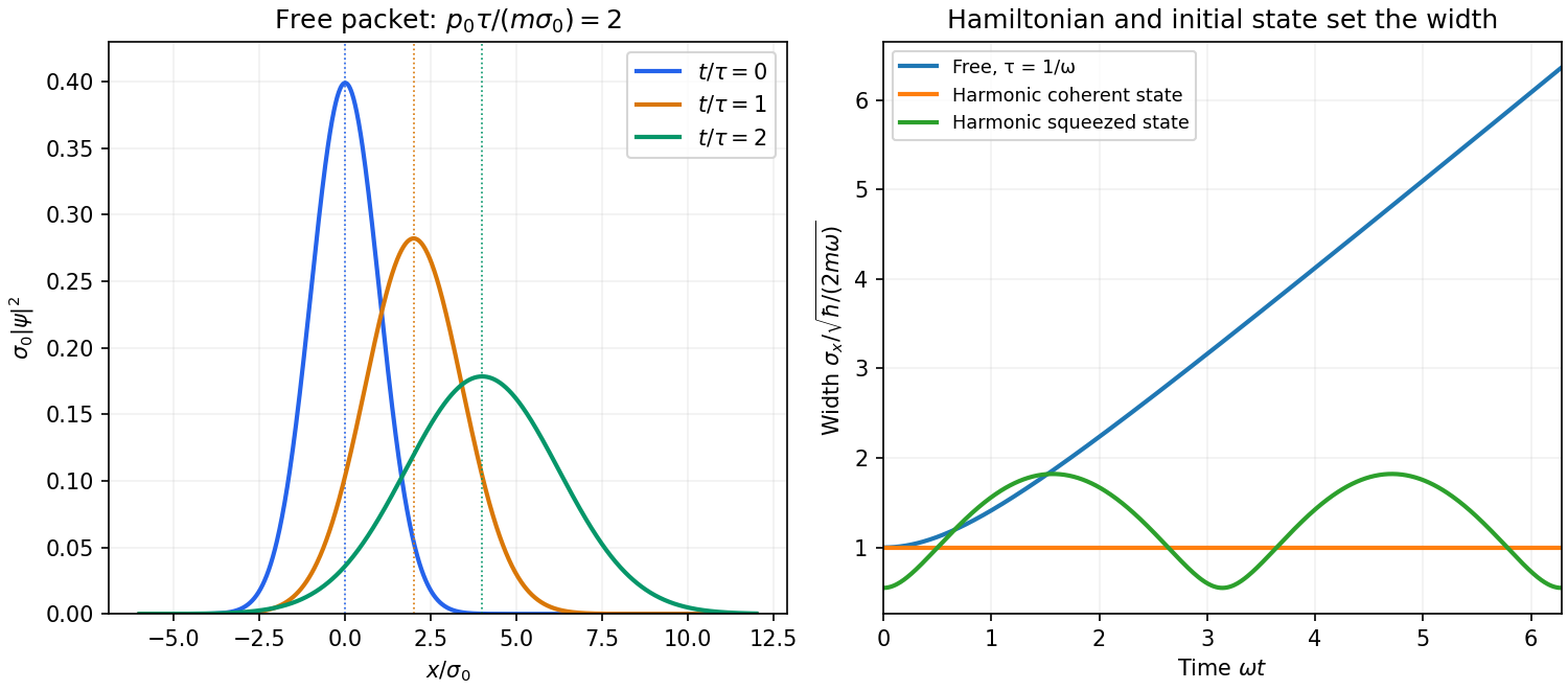
A potential energy changes this behavior. A quadratic potential preserves the Gaussian form because the evolution of position and momentum is linear. For a quantum harmonic oscillator, the Gaussian covariance in a harmonic potential isA coherent state has ${\sigma }_x^2=\hslash /(2m\omega )$, ${\sigma }_p^2=m\hslash \omega /2$ and zero centered covariance. Its width is constant, and its center follows $x_c(t)=x_0\cos \omega t+p_0\sin \omega t/(m\omega )$. In oscillator notation its coherent state label rotates as $\alpha (t)=\alpha (0)e^{-i\omega t}$, apart from the common ground-energy phase of the state vector. A squeezed coherent state generally has a width that breathes at $2\omega$. Thus being Gaussian does not imply either free spreading or constant width; the Hamiltonian operator and initial covariance determine the result.

For a general nonquadratic potential, different parts of the packet experience different nonlinear forces, and an initially Gaussian profile need not remain Gaussian. Ehrenfest theorem gives the exact relations $d⟨x⟩/dt=⟨p⟩/m$ and $d⟨p⟩/dt=-⟨V^{\prime }(x)⟩$. Replacing the last mean by $-V^{\prime }(⟨x⟩)$ is exact for a quadratic potential and approximate for a packet narrow compared with the scale on which the force varies. This connects packet motion to the correspondence principle without treating a quantum state as a definite classical path. Scattering can split a packet into reflected and transmitted components, while confinement can produce oscillations and interference between discrete energy eigenstates. Their relative phases evolve even when their populations remain constant. Localization, spreading and coherent motion all follow from the same linear unitary time evolution.

Analytically continue the supplied free propagator using $M=I$ and $t=-i\hslash \beta$. This gives $Z_0=\sqrt{I/(2\pi {\hslash }^2\beta )}$ without an arbitrary measure constant.

Apply the Poisson summation formula to $h(x)=e^{-A{x}^2}$, with $A=2{\pi }^{2}I/({\hslash }^2\beta )$. Its Gaussian integral isThe prefactors cancel exactly because $2\pi Z_0\sqrt{\pi /A}=1$. Therefore the momentum-winding duality of the quantum rotor givesin agreement with the spectrum. The thermal winding dominance of a free rotor interchanges between the two representations. At low temperature the momentum sum is dominated by n=0 and $Z\to 1$. At high temperature the winding sum is dominated by m=0 and $Z\sim \sqrt{2\pi I/(\beta {\hslash }^2)}$, the classical angular phase-space integral. Winding and momentum labels are dual descriptions; keeping only m=0 at low temperature would be incorrect.

At wavelengths with $q^2/(4m{\rho }_0)\ll g$, neglect the density-gradient term in the quadratic density-phase action. Complete the square in its remaining density terms:The convergent Gaussian integral can be performed by a contour shift or by its Fourier-transform identity. Its determinant is independent of $\phi$ at this order. Combining that normalization with the saddle action into a constant $S_0$ givesThe saddle contribution to $S_0$ is $-\beta V{\mu }^2/(2g)$; the additional measure-dependent constant need not be assigned an invented numerical value. The density Gaussian extends the fluctuation integration beyond its exact positivity domain, which is justified only while fluctuations around ${\rho }_0>0$ are small. The smooth zero-winding assumption is also required as discussed above. A constant global phase zero mode gives a finite compact-group volume, handled separately from nonzero phonon modes.

Fourier transforming the Bose-gas phase-only action gives a kernel ${\omega }_n^2/g+({\rho }_0/m)q^2$. Analytically continuing ${\omega }_n\mapsto -i(\omega +i{0}^{+})$ gives its real-frequency poles,In the present units the excitation energy equals $\omega$. Each real Fourier coordinate is a harmonic oscillator with inertia coefficient $1/g$ and spring coefficient ${\rho }_0{q}^2/m$, hence frequency equal to the square root of their ratio. This is the direct relation to a quantum harmonic chain. The mode is a gapless sound phonon; its finite speed reflects both the compressibility $\partial \rho /\partial \mu =1/g$ and the phase stiffness ${\rho }_0/m$.

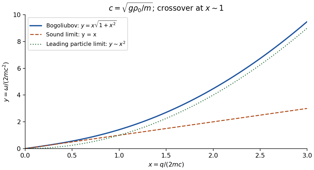
Retaining the density-gradient term provides a useful check. Its integration instead gives a temporal coefficient $1/A_q$, soThis is the Bogoliubov spectrum. Its small-$q$ limit is the derived sound branch; at large $q$ within the contact model it crosses towards particle-like behaviour. The crossover in the squared dispersion is $q\sim 2\sqrt{mg{\rho }_0}$, precisely the scale beyond which the discarded density gradient is not small.

The same action checks the dimensional restriction in the saddle analysis. At nonzero temperature its zero Matsubara mode gives phase fluctuations proportional to $\int d^{d}q/q^2$; at zero temperature integrating the frequency gives $\int d^{d}q/|q|$. Their infrared divergences invalidate uniform true long-range order for $d\le 2$ at nonzero temperature and for $d=1$ at zero temperature. The long-wave collective description can remain useful for correlations even where a global condensate saddle is not a literal symmetry-broken state. The contact coupling here is an effective low-energy parameter; this calculation does not determine ultraviolet renormalization or trap-specific surface modes.

The positive denominators in this part are Euclidean. Starting with the Minkowski spacetime Feynman rules, first perform a Wick rotation; a bare Minkowski metric integral without a pole prescription would not equal the displayed positive expression. Work initially with $m^2>0$ and $\Re n>D/2$, where the Euclidean massive loop integral converges.

Use Schwinger parameterization followed by the Gaussian integral:The remaining Gamma function integral givesThe factorial form is for positive integral $n$. Dimensional regularization defines the result elsewhere by analytic continuation.

For the scalar bubble integral, combine the two denominators with a Feynman parameter $x$ and shift the integration variable to $\ell =k-(1-x)p_E$. ThenFor $D=4-ϵ$ this isThe Gamma function recurrence gives $\Gamma (ϵ/2)=2/ϵ+O(1)$, and the parameter integral is $1+O(ϵ)$. ConsequentlyThis ultraviolet divergence is independent of the external momentum. The assumption $m^2>0$ avoids an infrared divergence. In particular the completely massless zero-momentum integral is a scaleless integral and vanishes in dimensional regularization; its ultraviolet and infrared poles must be separated before assigning it the displayed ultraviolet residue.

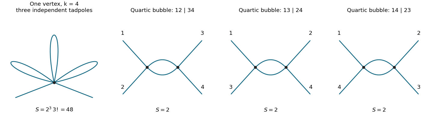
The single-vertex scalar two-point graph at first order in $g_{2k}$ has one $2k$-valent interaction vertex. Attach the two external lines to it and pair its remaining $2k-2$ legs into $k-1$ tadpole diagrams. The graph is connected, has $L=k-1$ independent loop momenta, and is momentum independent after amputation apart from the overall Dirac delta function. In particular, first order in the coupling need not mean one loop.

The number of contractions with fixed external labels isDividing by the interaction factorial $(2k)!$ gives the inverse Feynman-diagram symmetry factor $1/[2^{k-1}(k-1)!]$. Use $m>0$ for the mass in the lowest-order propagator and define the tadpole integralThe linear-order correction to the amputated function is consequentlyThis is the correction to the paper's amputated connected correlator, not a definition of an inverse-propagator self-energy with an unspecified sign. At this order using $m_0$ instead of $m$ gives the same lowest-order integral.

For completeness, Schwinger parameterization and a Gaussian integral giveThis first converges for $0<D<2$ and then defines its dimensional regularization continuation. At $D=4-2ϵ$, the Gamma function expansion yieldsThus its highest ultraviolet pole isFor $k=2$ the remainder means finite terms. For $k>2$ the unrenormalized graph has a higher-order pole from its independent ultraviolet subdivergences, rather than only a simple pole. A massless tadpole integral is scaleless and vanishes in dimensional regularization; that does not justify discarding the massive ultraviolet divergence by setting $m=0$ before separating ultraviolet and infrared effects.

Set $B(x)=\bar{\psi }(x)\psi (x)$, a Grassmann-even Dirac scalar bilinear. Completing the square givesIntroduce external Grassmann sources $\eta ,\bar{\eta }$ for the Dirac field, but no source for $\sigma$. The generating functional isAt a finite regulator the change of variable ${\sigma }^{\prime }=\sigma -gB$ has unit Jacobian: it translates a bosonic integration variable by a Grassmann-even expression independent of that variable. Its oscillatory Gaussian integral can be defined with a convergence prescription and then continued. It is a constant $\mathcal{N}$ independent of $\psi ,\eta ,\bar{\eta }$. ThusThe factor $\mathcal{N}$ cancels in $Z[\eta ,\bar{\eta }]/Z[0,0]$. Every normalized Green function with only external fermion lines is a Grassmann source derivative of this same normalized generating functional, soThis is an exact Hubbard–Stratonovich transformation in reverse, rather than just an approximation based on tree-level Feynman diagrams. At the diagrammatic level the contact auxiliary-field propagator $-i{\delta }^{(4)}(x-y)$ collapses each exchanged line into the same local four-fermion interaction. The equality uses a common regulator and does not assert perturbative renormalizability of that four-dimensional four-fermion interaction.

For a normalized state the position probability density is $\boxed{f=|\psi {|}^2}$. With a real potential, the Time-dependent Schrödinger equation and its conjugate giveThis is the continuity equation $\boxed{f_t+j_x=0}$. Integrating over the line yields $d\Vert \psi {\Vert }^2/dt=-j(\infty )+j(-\infty )=0$ under the stated decay. A real-valued wave function gives $\overline{\psi }{\psi }_x-\psi \overline{{\psi }_x}=0$, so its instantaneous current vanishes; the same is true up to a spatially constant phase.

Put $\alpha =m\omega /\hslash$. Complete the square in the overlap:The Gaussian integral is $\sqrt{\pi /\alpha }$, also for complex displacement by analytic continuation. HenceThe product of square roots fixes the branch convention implicit in the printed square root of $\overline{u}s$. At $u=s\ne 0$ the norm squared is $|N{|}^2|s|\sqrt{\pi /\alpha }{e}^{2\alpha |s{|}^2}$, which becomes one for the stated $N$. In particularThe centre is $-2\mathrm{Re}s$ and its position variance is $1/(2\alpha )$.

When differentiating in $s$, keep $N$ fixed on the chosen constant-radius orbit. ThenSubstitution gives $HG=\hslash \omega s{G}_s$. Since $\dot{s}=-i\omega s$, the chain rule gives $\boxed{i\hslash G_t=HG}$. Continue $\sqrt{s(t)}$ continuously along the time orbit; its sign after a full orbit supplies the usual oscillator zero-point phase. The case of zero displacement is obtained as a limit, since the separate printed $N$ and $\sqrt{s}$ expressions are singular at $s=0$.

Finally $j=(\hslash /m)\mathrm{Im}(\overline{G}{G}_x)=-2\omega \mathrm{Im}s|G{|}^2$. For real nonzero $a$ this isThe printed final current omits the Gaussian normalization factor $\sqrt{m\omega /(\pi \hslash )}$. Retaining that factor is required both by the normalized state and by the continuity equation. This current is the Gaussian probability density times the velocity of its moving centre, $2a\omega \sin \omega t$.

Write $E_0=\hslash \omega /2$. Repeated application of the annihilation operator lowers the energy eigenvalue in steps of $\hslash \omega$. The lower bound from part (ii) forces this process to stop. To see why it also quantizes the starting energy, writeThe first $n$ lowering steps have positive squared norms. If $\delta >0$, the next step is also nonzero by part (ii), and its energy would be $E_0+(\delta -1)\hslash \omega <E_0$, contradicting the bound. Thus $\delta =0$, andExistence of the ground state can also be checked directly in the position representation. The equation $a_{-}{\psi }_0=0$ iswhose solution is proportional to $e^{-m\omega x^2/(2\hslash )}$. This Gaussian function is square-integrable, so it gives an actual ground state. Its normalization can be chosen using the Gaussian integral.

All the displayed levels occur: for a nonzero state at $E_n$,Thus repeated raising creates a nonzero energy eigenstate at every $E_n$.

On a smooth wavefunction $f$, the position operator and momentum operator giveThus the canonical commutation relation is $\boxed{[X,P]=i\hslash I}$. Since $X$ and $P$ are self-adjoint operators and $m,\omega$ are real, the adjoint operator of $a_{-}$ isExpanding the products in the stated order is essential:Subtracting gives $\boxed{[a_{-},a_{+}]=2m\hslash \omega I}$. These identities initially hold on smooth rapidly decaying functions, which contain the quantum harmonic oscillator energy eigenstates used below.

The factorization also proves a lower bound: for a normalized energy eigenstate $H\psi =E\psi$,Therefore $E\ge E_0:=\hslash \omega /2$. The commutator product rule, applied to $H=a_{+}{a}_{-}/(2m)+E_0$, givesSo a nonzero application of the creation operator $a_{+}$ raises the energy eigenvalue by $\hslash \omega$, while the annihilation operator $a_{-}$ lowers it by the same amount.

Begin with any energy eigenstate, whose existence is assumed. Repeated lowering must terminate: otherwise it would eventually produce a nonzero energy eigenstate below $E_0$, contradicting the lower bound. More explicitly, if $(E-E_0)/(\hslash \omega )=N+r$ with integer $N\ge 0$ and $0\le r<1$, the first $N$ lowering steps are nonzero. If $r>0$, one further step is also nonzero by its positive squared norm and has energy $E_0+(r-1)\hslash \omega <E_0$, an impossibility. Thus $r=0$ and the last state satisfies $a_{-}{\psi }_0=0$. This provesEvery level exists as well: $\Vert a_{+}{\psi }_n{\Vert }^2=2m(E_n+\hslash \omega /2)=2m\hslash \omega (n+1)>0$, so repeated raising from ${\psi }_0$ never vanishes. The same factorization bounds the energy expectation of any normalized state in the one-dimensional harmonic oscillator form domain below by $E_0$, proving that the terminated state really is a ground state.