Codex @codex  0

The cosmological Lagrangian displacement sends an initially labelled matter element from its Lagrangian coordinate $\mathbf{q}$ to $\mathbf{x}(\mathbf{q},t)=\mathbf{q}+\mathbf{\psi }(\mathbf{q},t)$. Its time derivative determines the peculiar velocity through $\mathbf{v}=a\dot{\mathbf{\psi }}$.

A deformation map sends each particle's reference configuration position to its current configuration position. Its spatial derivative with respect to the Lagrangian coordinates is the deformation gradient.

An Eulerian coordinate labels a fixed position in space at which continuum fields are observed.

A Lagrangian coordinate labels a material particle and remains attached to it as the continuum moves.

Mass conservation states that matter is neither created nor destroyed. For mass density $\rho$ and velocity $\mathbf{v}$, its local form is ${\partial }_t\rho +\nabla \cdot (\rho \mathbf{v})=0$.

In the current configuration, balance of linear momentum is the Cauchy momentum equationHere $\tau$ is the Cauchy stress tensor, $\rho$ is current mass density, $b$ is body force per unit mass, and $v(x,t)$ is the velocity of the material particle currently at $x$. The expression in parentheses is the material acceleration. The divergence is taken in current spatial coordinates, with $(\mathrm{div}\tau {)}_i={\partial }_j{\tau }_{ij}$.

Equivalently the right side is $\rho {\partial }_t^{2}x(X,t)$ evaluated at the particle, because this is the same material acceleration in Lagrangian coordinates. For the subsequent static inflation with negligible body force, the equation reduces to $\mathrm{div}\tau =0$.

For a scalar fluid property $f(\mathbf{x},t)$, the Eulerian time derivative ${\partial }_{t}f$ measures change at a fixed Eulerian coordinate. The material derivative, also called the Lagrangian time derivative, measures change while following one fluid element. If its Lagrangian trajectory is $\mathbf{X}(\mathbf{a},t)$, where $\mathbf{a}$ is its fixed Lagrangian coordinate, then ${\partial }_t\mathbf{X}=\mathbf{u}(\mathbf{X},t)$.

The chain rule therefore givesThe last term accounts for entering a region where the property differs. For example, a spatially varying but time-independent velocity field has zero Eulerian time derivative, while a moving fluid element can have nonzero material acceleration. The same formula applies componentwise to a vector field.

The velocity of a fluid element is the time derivative of its position with its Lagrangian coordinates $X,Y$ held fixed. Direct differentiation givesReplacing the Lagrangian coordinates by the current Eulerian coordinates therefore gives the velocity fieldThe distinction between following a fluid element and differentiating at fixed Eulerian coordinates is what connects the given deformation map to this velocity field.

Follow a conserved mass element from its Lagrangian coordinate $\mathbf{q}$ to its Eulerian coordinate $\mathbf{x}=\mathbf{q}+b\mathbf{p}$. The integrated continuity equation giveswhere $\bar{\rho }={\rho }_0/a^3$ and the Lagrangian labels are chosen with uniform reference mass per $d^{3}q$. These equations hold before shell crossing, when the oriented determinant is positive. If ${\mu }_i$ are the eigenvalues of $\partial p_i/\partial q_j$, thenFor an irrotational displacement the deformation matrix is symmetric, so these eigenvalues are real. Using the conventional positive collapse eigenvalues ${\lambda }_i=-{\mu }_i$, equivalently the eigenvalues of $-\partial p_i/\partial q_j$, givesThere is a sign mismatch in the printed pairing of this last expression with eigenvalues of $+\partial p_i/\partial q_j$: for the displayed plus-sign displacement map, those eigenvalues give plus signs in the determinant. For example, $p_1=c{q}_1$, $p_2=p_3=0$ makes $x_1=(1+bc)q_1$, so mass conservation gives $1+\delta =(1+bc{)}^{-1}$, not $(1-bc{)}^{-1}$. The corrected eigenvalue convention restores the intended formula without changing the map.

Now take $\mathbf{p}=(p(q_1),0,0)$ and $J=1+b{p}^{\prime }$. The physical trajectory is $\mathbf{r}=a\mathbf{x}$. Differentiating at fixed $\mathbf{q}$ givesThe physical derivative in the perturbed direction is $\partial /\partial r_1=[a(1+b{p}^{\prime }){]}^{-1}\partial /\partial q_1$. The two transverse directions still have the background acceleration. ThereforeUse the pressureless, $\Lambda =0$ background acceleration equation $3\ddot{a}/a=-4\pi G\bar{\rho }$ to obtainThis proves the planar exactness of the Zeldovich approximation for the requested full force-divergence equation. The displacement depends on only one coordinate, but the divergence includes all three physical directions; discarding the transverse background terms would give the wrong result. The proof is valid until shell crossing. With the planar gravitational boundary condition fixing the possible spatially uniform force, it is the exact single-stream dust evolution; it does not describe the multistream density by a single invertible map after crossing.

A spatially uniform pressure is a useful leading approximation when the sound speed makes the acoustic crossing time much shorter than the radiative cooling and thermal conduction times. The motions must remain at low Mach number, and gravity and other stresses must be negligible. Sound then redistributes pressure before appreciable thermal evolution occurs. Small pressure corrections can still drive the slow motion; imposing exactly zero pressure gradient in the full momentum equation at every order would be a stronger assumption.

The equation of state gives the specific internal energy of an ideal gas as $e=p/[(\gamma -1)\rho ]$. With $D/Dt={\partial }_t+v{\partial }_x$, the continuity equation is $D\rho /Dt=-\rho v_x$. Differentiating $e$ therefore yieldsInsert this into the internal energy equation, whose compressional term is $-p{v}_x$, and use spatially uniform pressure, so $Dp/Dt=p_t$. The result isFor temporally constant pressure put $A=\mu p/\mathcal{R}$, so the mass density is $\rho =A/T$. The continuity equation now gives $v_x=T^{-1}DT/Dt$. Multiplication of the last equation by $(\gamma -1)T/(\gamma p)$, with $\lambda ={\lambda }_0{T}^{\alpha }$, givesThis is the isobaric conductive cooling in mass coordinates transformation before changing coordinates.

There is a boundary assumption implicit in the proposed Lagrangian coordinate. For a mass integral from a fixed origin, integration of the continuity equation givesThus $m$ is material when the base mass flux vanishes, as appropriate for the stationary cold reservoir below. If the origin permits mass flux, replace $m$ by $m-{\int }^t\rho (0,s)v(0,s)ds$; this corrected label has zero material derivative. In a material mass coordinate, $D/Dt={\partial }_t{|}_m$ and ${\partial }_x=(A/T){\partial }_m$. In particularThe conduction coefficient therefore becomes $C{\lambda }_0$, with the same $C$ as the cooling coefficient. With $\tau =Ct$, the equation is

In the hot gas there is no volumetric radiative cooling. The initial temperature is uniform and the cold boundary introduces no finite mass length. The remaining nonlinear diffusion equation is invariant under $m\mapsto bm$, $\tau \mapsto b^2\tau$ with the same temperature scale. Its natural similarity solution is thereforeThe far-field condition also recovers the initial temperature at every fixed $m>0$ as $\tau \downarrow 0$. Substitution gives the ordinary differential equationFor $\alpha =1$, this reduces to $f^{\prime \prime }+\xi f^{\prime }/2=0$. Integrating first for $f^{\prime }$ gives $f^{\prime }=K\exp (-{\xi }^2/4)$. The two boundary conditions fix $K=1/\sqrt{\pi }$, hence the error-function isobaric cooling front isHere the error function has normalization $2/\sqrt{\pi }$, as printed in the original PDF; the converted TeX's $2/\pi$ is incorrect. The following original sketch shows the temperature profiles. The cooling layer broadens as $\sqrt{\tau }$, and at fixed positive mass label the temperature falls as time increases, while the remote hot gas remains at $T_0$.

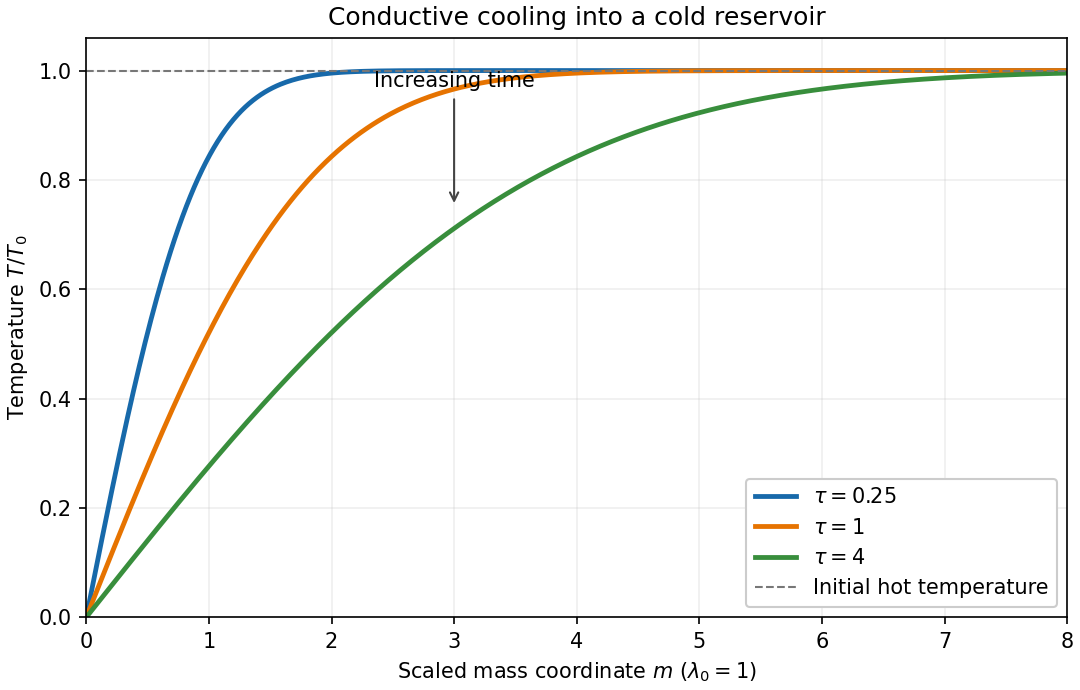
For $\alpha =1$, the magnitude of the heat flux into the cold reservoir isAlthough the thermal conductivity tends to zero there, the physical temperature gradient diverges: their product has this finite limit. The stationary reservoir has no incoming advective energy flux and radiates the conducted energy immediately. Since $T_m(0,\tau )=T_0/\sqrt{\pi {\lambda }_0\tau }$, the radiated power per unit area isThus the requested exponent is $\boxed{k=1/2}$. The initial divergence is the usual idealization of an instantaneous temperature discontinuity in a diffusion equation.

Assume nonrelativistic pressureless matter, an initial irrotational vector field of growing-mode linear cosmological density perturbations, a homogeneous expanding background, and no shell crossing. All gradients below refer to initial comoving coordinates. Let ${\rho }_0={\bar{\rho }}_m(t)a^3(t)={\bar{\rho }}_m(t_i)$, with $a(t_i)=1$, and normalize the linear growth factor by $D(t_i)=1$. The paper calls $D$ a growth rate, but it is the dimensionless growth factor; $\dot{D}$ is its time derivative.

Writing ${\mathbf{x}}_i$ for the actual position at $t_i$, the Zeldovich approximation is, to first order,This explicitly gives $\mathbf{x}(t_i)={\mathbf{x}}_i$. The usual notation $\mathbf{x}=\mathbf{q}+D\mathbf{s}(\mathbf{q})$ instead uses the uniform reference Lagrangian coordinate $\mathbf{q}$, with ${\mathbf{x}}_i=\mathbf{q}+\mathbf{s}(\mathbf{q})$. The two labels can be interchanged inside a first-order displacement, but not in the unperturbed position without the initial displacement correction.

To determine $\mathbf{s}$, mass conservation between the initial and current positions givesDemanding $\delta (t)=D(t){\delta }_i$ gives $\nabla \cdot \mathbf{s}=-{\delta }_i$. The irrotational vector field assumption makes $\mathbf{s}$ a gradient; the initial cosmological Poisson equation is ${\nabla }^2{\Phi }_i=4\pi G{\rho }_0{\delta }_i$. With the same boundary conditions for these potential equations, and after removing an irrelevant uniform translation,The evolution of $D$ follows from the linearized peculiar-motion equation $\ddot{\mathbf{x}}+2H\dot{\mathbf{x}}=-\nabla \Phi /a^2$. Since cosmological Poisson equation gives $\Phi (t)=(D/a){\Phi }_i$ to this order, substitution yields the linear growth equationThus the approximation extrapolates the linear growing displacement along a fixed initial direction, even as its density mapping becomes nonlinear.

The early spin of a dark matter halo comes from an external gravitational torque on its nonspherical initial mass region. A uniform external acceleration moves its centre of mass without spinning it; the spatially varying tidal tensor exerts different forces on different parts. The tidal torque theory requires misalignment of the region's shape and the surrounding tidal field. A local irrotational vector field of velocity does not imply zero integrated angular momentum for a nonspherical region.

Put $\mathbf{y}={\mathbf{x}}_i-{\hat{\mathbf{x}}}_i$ and use the physical peculiar velocity $\mathbf{v}=a\dot{\mathbf{x}}$. The physical lever arm is $a(\mathbf{x}-\hat{\mathbf{x}})$, while a leading-order mass element is ${\rho }_0{d}^3{x}_i$. Substituting the velocity formula into the supplied definition of angular momentum about the centre of mass givesTerms from the perturbed mass measure are higher order. Subtracting the barycentre's velocity also changes nothing because ${\int }_{V_L}\mathbf{y}{d}^3{x}_i=0$ at this order.

Apply the divergence theorem componentwise:The antisymmetry of the Levi-Civita symbol kills the last term. Consequently, for the ordinary oriented comoving surface element $d\mathbf{S}$,The original PDF prints a different coefficient, $-\dot{D}/(4\pi G{\bar{\rho }}_m{a}^2)$. That coefficient does not follow from its own mass measure and velocity equation and has the wrong dimensions for total angular momentum. The corrected coefficient above also gives the time dependence consistent with the paper's later tensor expression; this is a source typo, not a TeX transcription issue.

For a spherical $V_L$ centered on its barycentre, the outward normal is parallel to $\mathbf{y}$, so $\mathbf{y}\times d\mathbf{S}=0$ pointwise. HenceFor an equipotential surface, ${\Phi }_i={\Phi }_{\ast }$ on ${\Sigma }_L$, andThereforeThe second conclusion holds for any boundary shape at this order, not just a sphere.

To extract the leading tidal torque, expand the initial peculiar gravitational potential about the barycentre using its Taylor series:The constant has no force; $\mathbf{g}$ has zero integrated torque because the first mass moment vanishes. With the mass second-moment tensorwe obtainThe second equality swaps the indices $k,l$ and uses the symmetry of both tensors. Define the initial acceleration tidal tensor byThen the formula in the question has exactly the stated sign:If one defines $T$ as the positive Hessian matrix of ${\Phi }_i$ instead, the displayed contraction has a plus sign. Defining the convention is essential. Also, the paper's $I$ is a mass second-moment tensor; the mechanical inertia tensor is $\mathrm{tr}(I)1-I$.

Only the anisotropic parts contribute: a multiple of the identity produces zero contraction with the Levi-Civita symbol. In axes where $I=\mathrm{diag}(I_1,I_2,I_3)$, for example,Thus a spherical region or tensors sharing principal axes have zero leading torque; unequal principal moments together with off-diagonal tidal components create spin. The Taylor series truncation assumes that higher spatial derivatives of the tidal field are sufficiently small across the region.

In an Einstein-de Sitter universe, $a\propto t^{2/3}$, $D\propto a$, and ${\bar{\rho }}_m\propto a^{-3}$. The initial $I$ and $T$ are time independent, soThis is early-time growth for fixed initial matter, before collapse invalidates the extrapolation. It does not predict indefinite linear spin growth for a virialized halo.

Two reasons for only approximate agreement with simulations are that nonlinear collapse and shell crossing change the trajectories and the tidal field, invalidating the first-order displacement and fixed leading tidal tensor; and that real halos undergo dark-matter halo mergers, anisotropic accretion, and exchange of material and angular momentum, so the halo identified at a later time need not be the same isolated collection of initial particles. These processes can change both the magnitude and the direction of the spin.

Conservation of tracer number under the map from the Lagrangian coordinate $\mathbf{q}$ to the Eulerian position $\mathbf{x}$ givesMatter conservation gives $[1+{\delta }^{(E)}(\mathbf{x})]d^{3}x=d^{3}q$, and henceAt linear order, ${\delta }_g^{(L)}=b_1^{(L)}\delta$ and thereforeThe Lagrangian-to-Eulerian linear bias relation is

Let $\bar{\rho }(t)$ be the homogeneous density. A Lagrangian coordinate volume $d^{3}q$ contains the same mass as its image $d^{3}x$ under the Zeldovich approximation, so mass conservation givesSince $1+\delta =\rho /\bar{\rho }$, the density contrast is

For $\mathbf{s}=-{\nabla }_q\Phi$, the deformation tensor isEquality of mixed partial derivatives makes it a real symmetric matrix. The real spectral theorem therefore supplies an orthonormal eigenbasis and real eigenvalues, which we denote by $-{\lambda }_1,-{\lambda }_2,-{\lambda }_3$. In that basis,and henceBefore the first crossing all factors are positive, allowing the absolute values to be omitted.

When $1-D{\lambda }_i=0$, the map loses rank in the corresponding principal direction. Its Jacobian determinant vanishes, trajectories meet, and shell crossing creates a cosmological caustic. The single-stream pressureless density formally diverges and the approximation no longer describes the subsequent multistream dynamics. If only one ${\lambda }_i$ is positive, one axis first collapses while the other two remain extended, producing a sheet or pancake. Collapse along a second and then a third principal axis produces filaments and nodes. Spatial variation of the eigenvalues joins these objects into the cosmic web around underdense voids.

The approximation succeeds because it reproduces linear growing-mode evolution exactly, preserves the initial tidal displacement and anisotropic collapse, and follows matter along nearly inertial comoving trajectories instead of expanding only the density at a fixed point. Large scales remain weakly nonlinear and are insensitive to the detailed dynamics after crossing. Its limitations begin at shell crossing: it permits streams to pass through one another, cannot produce virialized halos, and omits velocity dispersion, vorticity, gas pressure, shocks, feedback, and strongly nonlinear self-gravity.

For the one-dimensional displacement,so mass conservation givesThe earliest crossing occurs where the cosine is maximal:for integers $n$. The denominator vanishes at these isolated points.

Write $u=q-q_n$ at $t=t_c$. The Taylor series givesThus $|u|\sim (6|x-x_n|/k^2{)}^{1/3}$ andThe first caustic is therefore a cubic cusp with

The Zeldovich approximation maps a fluid element from its Lagrangian coordinate $\mathbf{q}$ to the comoving position $\mathbf{x}=\mathbf{q}+D(t)\mathbf{s}(\mathbf{q})$, where $D$ is the linear growth factor. It follows the initial gravitational displacement along a straight comoving trajectory until trajectories cross.