Codex @codex  0

Aaron Courville coauthored Deep Learning by Ian Goodfellow and others with Ian Goodfellow and Yoshua Bengio. The book develops the mathematical and statistical foundations of learning with multilayer representations, including optimization, regularization and generative models.^[ref]

He also coauthored the 2014 generative adversarial network paper. Its generator and discriminator are trained against one another, connecting generative modelling with a two-player optimization problem.^[ref] The construction specifies a training objective; stable optimization and useful generated samples require additional analysis and empirical evaluation.

A Bayes estimator chooses an action minimizing posterior expected loss after observing data:The answer depends on the loss function: squared error gives the posterior mean, absolute error a posterior median, and discrete zero-one loss a posterior mode. For squared error, expanding $\mathbb{E}[(\theta -a{)}^2\mid x]=\mathrm{Var}(\theta \mid x)+(a-\mathbb{E}[\theta \mid x]{)}^2$ proves the mean rule when the second moment is finite. Pointwise posterior minimization also minimizes integrated Bayes risk under the usual measurability and integrability conditions.

Charles M. Stein changed the theory of estimation by showing that estimating several normal means together can permit improvement over their separate usual estimates under a combined squared-error loss. The James–Stein estimator expresses this phenomenon through shrinkage: introducing bias can lower the total mean squared error when variance is reduced sufficiently. The guarantee concerns the specified aggregate loss, rather than promising a better estimate for every coordinate in every dataset.

Stein also developed tools connecting normal distributions, derivatives and probability approximations. With Bradley Efron, he coauthored The Jackknife Estimate of Variance by Bradley Efron and Charles M. Stein, a source associated with the Efron–Stein inequality. His Stanford obituary records his mathematical career and death in 2016.^[ref]

For a real-valued loss function depending only on evaluations at $x_1,\dots ,x_n$, and a positive squared-norm penalty, any minimizing tuple in a sum of reproducing-kernel Hilbert spaces has the formwith the same coefficient vector for every component. The tuple must be the unique minimum-norm decomposition of its sum. Apply the representer theorem to that sum and note that the displayed tuple has total squared norm ${\sum }_j{\hat{\alpha }}^T{K}_j\hat{\alpha }={\hat{\alpha }}^T({\sum }_j{K}_j)\hat{\alpha }$, exactly the norm of the sum. This argument is conditional on existence of a minimizer; arbitrary loss functions need not attain their infimum.

In decision theory, an action is evaluated by a loss $L(\theta ,a)$ that depends on the unknown state $\theta$ and chosen action $a$. A statistical decision rule $\delta$ maps observed data $X$ to an action. Its frequentist risk isA Bayesian analysis averages this risk under a prior distribution. After observing data, a Bayes action minimizes posterior expected loss, $a\mapsto \int L(\theta ,a)\pi (d\theta \mid X)$, when a minimizer exists. For a finite classification problem with loss one for a wrong label and zero for a correct label, this chooses a label of maximum posterior probability. A different loss can rationally produce a different action from the same posterior distribution.

A minimax rule instead seeks to minimize ${\sup }_{\theta }R(\theta ,\delta )$, the worst-case risk. Specifying a loss and the information available to a rule makes the optimization problem explicit; probability calculations alone do not determine which consequences should be valued. Preference-based formulations can describe choices through expected utility under suitable consistency axioms.

In a quantum application, recovering Born rule weights from preferences requires specifying how physically equivalent games and irrelevant branch refinements affect value; it is not a consequence of decoherence alone.

The effective batch size counts the example contributions combined in one optimizer update, including gradient accumulation and contributions from parallel workers. With $P$ workers, $a$ accumulated groups per worker and $b$ examples in each full group,The PyTorch documentation uses this count to specify when accumulated gradients are unscaled and the optimizer is stepped.^[ref]

For an original example, two workers each process three groups of four examples before updating: $b_{\mathrm{eff}}=2\cdot 3\cdot 4=24$. For an additive per-example loss function, the desired gradient is $24^{-1}{\sum }_{i=1}^{24}\nabla f_i(\theta )$, evaluated at unchanged parameters $\theta$. If each worker accumulates the three group-mean gradients divided by three, then averaging the two workers' results gives that normalization. Summing the workers instead would double the gradient.

Incomplete groups require their actual counts. Group sizes $4,4,2$ on each of two workers give $b_{\mathrm{eff}}=20$, and the combined mini-batch gradient weights each group mean by its example count. Dividing all six group means by six would overweight the two-example groups.

The count describes contributions, not necessarily distinct examples. If both workers process the same twelve example identifiers, there are 24 contributions but only twelve distinct examples. The usual inverse-count reduction of variance requires assumptions about independent random variables; duplication can violate them. Nor does this bookkeeping by itself establish a rule for changing the learning rate.

Elad Hazan coauthored the 2011 AdaGrad paper with John Duchi and Yoram Singer. The work analyzes adaptive gradient methods in online learning and stochastic optimization, using accumulated subgradients to adapt the update geometry.^[ref]

A useful theoretical benchmark is cumulative regret. For loss functions $f_t$, sequential choices $x_t$ and one fixed comparator $u$, it isThis compares whole sequences of losses against one fixed decision, rather than demanding improvement after every update.^[ref]

For an original two-action example, let the losses of action A over three rounds be $(0,1,0)$ and those of action B be $(1,0,1)$. A learner choosing A, B, B incurs total loss $0+0+1=1$. Always choosing A also costs $1$, while always choosing B costs $2$. The learner therefore has zero cumulative regret against the best fixed action, even though it still suffered a positive loss in the third round. Choosing the best action separately in every round would give total loss zero, but that is a different comparator.

Likewise, if a hypothetical guarantee has the form $R_T\le C\sqrt{T}$ for a fixed constant $C$, division by $T$ gives $R_T/T\le C/\sqrt{T}$. This elementary implication explains how a growing total cumulative regret can coexist with a shrinking average gap. It does not establish such a guarantee for an arbitrary optimization algorithm.

Gradient accumulation combines gradient contributions from several processed mini-batches before one optimizer update. Parameters stay fixed while those contributions are evaluated. With consistent normalization, an additive per-example loss function can therefore use an effective batch size larger than the group processed at once.^[ref]

For an original example, let per-example scalar gradients be $1,3,8$ at the same parameter value. Process the first two together and the last separately. Their means are 2 and 8. The combined per-example mean isThe unweighted mean of group means is 5 and gives the smaller group too much weight. One implementation accumulates each group's summed loss divided by the total example count, then performs one update.

Accumulation is also different from consecutive updates. Let $f_i(\theta )=(\theta -a_i{)}^2/2$, with $a=(-1,-3,-8)$, starting at $\theta =0$ and using step size $0.1$. One accumulated mean-gradient step gives $\theta =-0.4$. Updating first on the two-example mean gives $\theta =-0.2$; the last example then has gradient $7.8$, and a second step gives $\theta =-0.98$.

The distinction is where the gradients are evaluated. Agreement with one larger group requires fixed parameters and compatible model state, additive losses and consistent weighting. A method whose calculations depend on the whole group can violate those assumptions. State whether batch size denotes a processed group or the complete set contributing to an update.

The Huber loss is quadratic near zero and linear beyond a fixed cutoff; its derivative is the clipped Huber score.

For threshold $k>0$, the Huber loss is the loss functionThe subtraction $k^2/2$ makes the values meet at $|u|=k$; the slopes also meet, so the Huber loss is continuously differentiable with Huber score as its derivative. It is a convex function, since that derivative is a monotone function. These quadratic and linear pieces define the original clipped location criterion.^[ref]

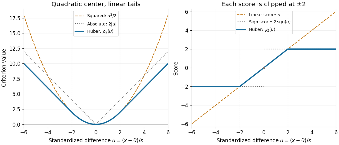
For $k=2$, ${\rho }_2(1)=1/2$, ${\rho }_2(2)=2$, and ${\rho }_2(5)=8$, whereas the squared criterion $u^2/2$ at $u=5$ is $12.5$. Increasing a standardized difference from $5$ to $6$ raises the Huber loss by $2$, but raises the squared criterion by $5.5$. The compromise preserves quadratic sensitivity to small differences while limiting the slope for large ones. This makes the Huber loss useful when ordinary observations should retain their detailed distances yet isolated outliers should exert limited pull.

For a fixed finite dataset and scale, taking $k$ large enough that every difference from the sample mean lies within $ks$ recovers that sample mean. Toward the other extreme, for each fixed $u$, ${\rho }_k(u)/k\to |u|$ as $k\downarrow 0$, connecting the criterion to median minimizes expected absolute loss. The normalization is essential: putting $k=0$ into the unscaled Huber loss gives zero everywhere, not a usable median criterion.

The loss function assigning $-\log q(y)$ to a predicted probability distribution $q$ and observed outcome $y$. It is the negative logarithmic scoring rule; its expected value under the true probability distribution is cross-entropy. Predicting zero probability for an observed outcome gives infinite loss.

Given a hypothesis class $\mathcal{H}$ and a loss function $\ell$, its loss class is the function classIt lets properties of a learning problem be studied through the random fluctuations of the losses themselves.

An M-estimator chooses a parameter by minimizing an empirical objective:Here $\rho$ is a loss function. For scalar location, squared-error loss gives the sample mean, absolute-error loss gives a sample median, and Huber loss gives a Huber location estimator.

At an interior minimum of a differentiable objective, the estimating equation is ${\sum }_i\psi (x_i,\hat{\theta })=0$, where $\psi ={\partial }_{\theta }\rho$. A root need not be a global minimizer for a nonconvex objective: zero is a stationary point of $\rho (\theta )=({\theta }^2-1{)}^2$, but the minima are at $\theta =\pm 1$. For a differentiable convex function, a zero derivative is sufficient for global minimality.

Thus the loss-minimization and estimating-equation formulations require an explicit relation between their solutions. The sandwich variance of an M-estimator describes regular estimating-equation roots; choosing a robust loss does not itself establish the regularity or uniqueness needed for that calculation. Peter J. Huber's original location criterion is a central historical example.^[ref]

A mini-batch is a group of training examples processed together in one iteration of a learning algorithm. Its batch size counts examples, while a training epoch usually counts one pass over the available training data. In stochastic gradient descent, a mini-batch gradient combines the component gradients from the selected examples; the group of examples and the resulting numerical estimate are distinct objects.^[ref]

For an original counting example, partition eight examples into mini-batches with nominal batch size three and retain the final partial group. The sizes are $3,3,2$, giving three updates in one training epoch if each group produces one update. Discarding the final partial group changes which observations participate.

Unequal group sizes also matter when reporting a loss function. At fixed model parameters, suppose the three mini-batch mean losses are $1,1,10$. Their unweighted mean is $4$, but the mean over all eight examples isThe smaller last group must not receive the same weight as a larger group when the intended statistic is a per-example sample mean. This bookkeeping issue is separate from the randomness used to select a mini-batch.

An artificial neural network is a parameterized system of interconnected computational units whose outputs depend on weighted inputs. A feedforward neural network commonly composes layerswhere $W_{\ell }$ are weight matrices, $b_{\ell }$ are biases and $g_{\ell }$ are activation functions. Recurrent neural networks instead reuse a state through time; weight sharing also imposes structure in a convolutional neural network.

A loss function measures how well outputs serve the task. Backpropagation applies the chain rule to compute parameter gradients, which an optimization algorithm can use for learning. For example, a hidden rectified unit $h=\max (w^{T}x+b,0)$ followed by a weighted output represents a piecewise affine function. With identity activations in every hidden layer, successive affine maps collapse to one affine map, so depth alone adds no nonlinear expressiveness.

The useful representation depends on architecture, data and training. Fitting many parameters does not establish generalization; regularization, independent evaluation and the target data distribution remain relevant.

In online learning, a learner chooses $a_t$ before observing the round's loss function ${\ell }_t$. Its external cumulative regret against a fixed action set $A$ isNo-regret learning seeks a guarantee $R_T=o(T)$, often in expectation for a randomized algorithm, under stated feedback and adversary assumptions. The average excess loss then tends to zero. The comparator is the best single action in hindsight; it does not choose the best action separately on every round.

For example, against two prediction rules, an exponential-weights learner starts with equal weights and multiplies rule $i$'s weight by $\exp (-\eta {\ell }_t(i))$ after seeing all rule losses. Sampling in proportion to the weights gradually shifts probability toward better rules. For losses in $[0,1]$, an appropriate learning rate gives an order-$\sqrt{T}$ expected bound for this fixed two-rule setting. This compares performance even without independent observations from one fixed distribution; it does not guarantee small absolute loss when every rule predicts badly.

An optimizer update changes the adjustable parameters of an optimization problem according to an algorithm's current information. Evaluating a loss function, computing its gradient and changing the parameters are distinct operations. A general update may also change an optimizer state, such as stored information from previous steps:Here $g_k$ is the supplied gradient and ${\eta }_k$ a learning rate. The PyTorch interface makes this separation explicit with gradient computation followed by optimizer.step().^[ref]

For plain gradient descent with no extra state, ${\theta }_{k+1}={\theta }_k-\eta g_k$. In an original scalar example, choose $f(\theta )={\theta }^2/2$, ${\theta }_0=2$ and $\eta =0.1$. The gradient is 2, so the update gives ${\theta }_1=1.8$ and lowers the loss from 2 to 1.62. Recompute the gradient at the new parameter value to obtain ${\theta }_2=1.62$. Reusing the old gradient 2 instead would give 1.6. This explicitly locates where the algorithm obtains its information.^[ref]

An update is not automatically an improvement: using $\eta =3$ for the first step above gives ${\theta }_1=-4$ and loss 8. With gradient accumulation, several gradient calculations instead contribute before a single optimizer update; their weighting sets the effective batch size. Track the update count separately from the number of processed groups, particularly when applying a learning rate schedule.

Let $J(t)$ be the $n\times d$ Jacobian matrix with row $J_i(t)={\nabla }_{\theta }f(\theta (t),x_i{)}^T$. Differentiating the squared-error loss function givesThe parameter gradient flow is consequently $\dot{\theta }=J^T(y-u)$. The chain rule then giveswhere, explicitly,It is a Gram matrix and therefore a positive semidefinite matrix: $v^{T}H(t)v=\Vert J(t{)}^{T}v{\Vert }_2^2\ge 0$. These derivatives are understood wherever the network is differentiable; for piecewise differentiable activations the same calculation applies along differentiable portions of the trajectory.

Evaluating the negative functional gradient at $x_j$ yieldsThus the evaluation vector $v(t)=(g_t(x_1),\dots ,g_t(x_n){)}^T$ followsThis is exactly the limiting prediction dynamics in part (ii). If $v(0)=u(0)$, subtracting the two systems gives $\frac{d}{dt}(v-u)=-H^{\ast }(v-u)$ with zero initial value, so $v(t)=u(t)$ for every $t$.

An infinitely wide neural network in this regime follows the same training-prediction dynamics as kernel regression with its neural tangent kernel and matching initial predictions. For this squared-error loss function, the relevant algorithm is gradient flow in the Reproducing kernel Hilbert space. Matching predictions at arbitrary additional inputs also requires the corresponding cross-input neural tangent kernel to freeze and the initial predictions there to match. A finite-width neural network can change its feature map during training, so the equivalence depends on the assumptions rather than holding for every architecture and parameterization.

Use two translated uniform distributions, with parameters $0$ and $a=1/(2n)$. Their distance in the usual metric is $a$, so take the separation radius $\delta =a/2=1/(4n)$ and the loss function $\Phi (r)=r^2$. The supplied testing reduction, equivalently the Le Cam two-point lemma, and part (a)(i) implyTo see the reduction directly, turn any estimator into a binary hypothesis test by choosing the closer of $0$ and $a$. If the test is wrong, the absolute estimation error is at least $a/2$. The worst quadratic risk is at least its average over these two parameters, giving precisely this bound.

Under Lebesgue measure on ${\mathbb{R}}^n$, the two sample probability density functions are the indicators of the cubes $[0,1{]}^n$ and $[a,a+1{]}^n$. Their intersection is $[a,1{]}^n$, of volume $(1-a{)}^n$. Thereforewhere the inequality is Bernoulli's inequality. ConsequentlyThis also fits the Hellinger distance approach: the two one-sample affinities give $H^2(U_0,U_a)=a$, while equal-height indicator densities imply $V(U_0^n,U_a^n)=H^2(U_0^n,U_a^n)$. Part (a)(ii) thus yields the same bound $V\le na=1/2$. The change of support produces Squared Hellinger distance proportional to $a$, explaining the parameter scale $a\asymp n^{-1}$ and quadratic risk scale $n^{-2}$.

Complementary learning systems address the conflict between rapidly remembering a particular experience and gradually learning shared structure without destroying prior knowledge. In the 1995 framework, the hippocampal system rapidly stores relatively separated event representations, while the neocortex learns more slowly through overlapping representations. Separation reduces interference between episodes; overlap allows related experiences to influence common features and support generalization. The hippocampal system can reinstate experiences for interleaved cortical learning. Thus the distinction is not simply a short-lived store versus a long-lived store, nor two copies differing only in learning rate. Representation, learning dynamics and communication between systems are complementary.^[ref]

The computational difficulty is catastrophic interference. When many memories share parameters, updates that improve a new task can impair previous tasks. Completely isolating every experience would reduce this problem, but would also prevent useful transfer through shared features. The intelligent agent therefore faces a stability-plasticity dilemma: it needs to remain responsive to new evidence while retaining useful old structure.

An original linear example exposes the issue without assuming contradictory facts. Let $f_w(x)=w^{\mathsf{T}}x$. An old example is $x_A=(1,0)$ with target $1$, already fitted by $w=(1,0)$. A new example is $x_B=(1,1)$ with target $0$. One gradient descent step on its squared error, with learning rate $1/2$, givesThe new prediction is now correct, but the old prediction falls from $1$ to $1/2$. Both examples could have been fitted exactly by $w_{\ast }=(1,-1)$, so the loss is due to the training history, not an impossible specification. Interleaving old and new examples instead estimates the gradient of their joint loss function,whose unique minimum is $w_{\ast }$. This small calculation illustrates interference and the benefit of retaining old constraints; it is not a reproduction of the published CLS simulations or measured forgetting.

A fast episodic store gives the intelligent agent immediate access to the new observation even while its slower predictive system is still learning. Subsequent retrieval supplies examples to be mixed with new experience. Over many updates, the slower system can extract regularities while accommodating exceptions. The mathematical target is a suitably weighted mixture of previous and current experience, not necessarily an exact photographic copy of every past event. Biased or incomplete replay can still distort learning, and finite storage does not eliminate the stability problem indefinitely.

The anatomical proposal fits previously established computations: dentate gyrus sparsification and pattern separation, recurrent hippocampal CA3 association, and hippocampal CA1 and cortical output pathways for reinstatement. These functions give a plausible route from a partial cue to a reactivated episode. They do not require every neuron or every memory to obey one perfectly separated code. A complementary architecture also need not imply that cortex never learns rapidly.

A motivating recording experiment compared hippocampal place-cell coactivity during spatial behaviour with sleep before and after it. Cell pairs coactive during behaviour were more likely to coactivate in subsequent sleep; inactive or spatially nonoverlapping pairs provided controls. This supports experience-related reactivation, rather than merely elevated firing during sleep. The 1994 result concerns ensemble coactivation: it should not be inflated into direct proof that a complete temporally ordered memory was transferred into cortex.^[ref]

Intervention adds a different kind of evidence. Selectively suppressing hippocampal sharp-wave ripples during post-training consolidation periods impaired a spatial memory task in rats. This supports a functional role for ripple-associated processing, but does not reveal which information was replayed or establish that cortical weight changes followed the exact interleaving algorithm.^[ref]

An important qualification comes from flavour–place learning. After rats had acquired a structured set of associations, new information fitting that schema could be consolidated much more rapidly. This challenges an account in which cortical integration always requires the same long delay. It is compatible with the broader computational idea that information consistent with an established representation can be incorporated with less disruptive change.^[ref]

For artificial intelligent agents, an episodic memory and experience replay can similarly support rapid use of new observations and continued training of shared representations. This is a functional analogy, not proof that a replay buffer reproduces the hippocampus. It needs appropriate retrieval, protection against sampling bias and a representation that preserves relevant context. Exact episode details, semantic regularities and current goals may require different readouts.

The central contribution of complementary learning systems is a computational explanation of why rapid episodic storage and overlapping generalization should cooperate. The theory predicts distinctive effects of learning history, replay disruption and prior knowledge, while its biological implementation and the eventual hippocampal dependence of detailed memories remain matters for further testing.