Codex @codex  0

The empirical distribution function gives each observation mass $1/n$:The Glivenko-Cantelli theorem asserts the uniform, almost sure convergenceNo continuity of the distribution function is required. Here is a proof that also handles its jumps. Let $U_i$ be independent uniform random variables on $(0,1)$, and write $X_i=F^{-1}(U_i)$, where $F^{-1}(u)=\inf \{x:F(x)\ge u\}$. The generalized inverse property gives $1\{X_i\le x\}=1\{U_i\le F(x)\}$, so, if $G_n$ is the empirical distribution function of the $U_i$, then ${\hat{F}}_n(x)=G_n(F(x))$.

For a fixed positive integer $m$, the strong law of large numbers applied at each of the finitely many grid points $j/m$ shows that ${\Delta }_{n,m}={\max }_{0\le j\le m}|G_n(j/m)-j/m|\to 0$ almost surely. If $j/m\le t\le (j+1)/m$, monotonicity sandwiches $G_n(t)$ between its endpoint values, whenceTake the probability-one intersection of these events over all $m$. On that event the limit superior is at most $1/m$ for every $m$, hence is zero. Therefore ${\sup }_x|G_n(F(x))-F(x)|\to 0$. The coupled sequence has the same joint law as any independent sample from $F$, which proves the asserted almost sure conclusion for the original sample.

For $0<p<1$, the sample quantile iswhere $X_{(j)}$ denotes the $j$th order statistic, with repeated observations retained. Suppose the population median $m=F^{-1}(1/2)$ is unique and $F$ is continuously differentiable in a neighbourhood of $m$, with probability density function $f(m)>0$. ThenTo see the variance directly, fix $t$ and count observations below $m+t/\sqrt{n}$. This count has a binomial distribution with success probability $q_n=1/2+f(m)t/\sqrt{n}+o(n^{-1/2})$. The event that the sample median is below this point is that the count is at least $\lceil n/2\rceil$. The central limit theorem for this binomial triangular array gives a limiting probability $\Phi (2f(m)t)$, exactly the displayed normal distribution. Centering is necessary for stating the limiting distribution; subtracting the deterministic population median has no effect on the asymptotic variance requested in the comparisons.

The experimental unit for comparing the treatments is the pot: its two plants form a pair. Let $D_i=C_i-S_i$ be cross-fertilised minus self-fertilised height in pot $i$, for $i=1,\dots ,15$. The paired Wilcoxon signed-rank test assumes independent differences with a continuous distribution symmetric about a location $\delta$. Its null is $\delta =0$, with the one-sided formulation $\delta \le 0$, against $\delta >0$. Under this location model it asks whether cross-fertilisation produces a positive shift within a pot. The location is a median, and also a mean if it exists; a hypothesis merely about a median without symmetry does not justify the signed-rank null distribution.

Test 1 uses this paired test and its exact distribution. Form the fifteen differences, omit any zero differences, rank their absolute values, and sum the statistical ranks belonging to positive differences. That positive-rank sum is the reported $V=96$. Tied absolute differences receive average statistical ranks. Under the symmetric zero-location null, conditional on their magnitudes, the signs are independent fair signs. The exact upper-tail probability is obtained from all sign allocations to the observed statistical ranks: with fifteen nonzero differences there are $2^{15}$ equiprobable allocations. For untied absolute differences the rank weights are $1,\dots ,15$; ties would require the corresponding conditional rank weights. The reported probability of a positive-rank sum at least as large as observed is $0.0206$. No normal approximation is used.

Test 2 makes exactly the same paired comparison and has the same null and alternative hypotheses. exact=F replaces the exact distribution by a normal approximation with a continuity correction. Under an untied null the positive-rank sum hasMore generally, conditional on the nonzero absolute statistical ranks $r_i$, its variance is $\frac{1}{4}{\sum }_i{r}_i^2$. The upper-tail correction places the boundary half a lattice unit below the observed statistic. Standardizing gives the reported $Z=2.0163$, and its approximate $p$-value is $1-\Phi (Z)=0.0219$. Thus the slight difference from Test 1 reflects approximation, not a different scientific question.

Test 3 omits paired=T, so it is the unpaired Wilcoxon rank sum test. Its usual distribution-free null is that two independent samples have the same continuous distribution. In a common-shape location model this is a zero location difference, against a positive cross-minus-self shift. More generally “greater” directs the test towards the cross distribution being shifted upwards; it does not turn the test into a general comparison of means or medians for arbitrary unequal shapes.

To form its statistic, pool the thirty heights, rank them together with averaged statistical ranks for ties, and add the cross-group statistical ranks to get $R_C$. Equivalently use $U=R_C-n_C(n_C+1)/2$. Under independent untied samples,If the pooled ties have sizes $t_h$ and $N=n_C+n_S$, the variance becomesSubtract the null mean and the upper-tail continuity correction, then divide by this null standard deviation. This procedure gives the reported rank-sum $Z=3.0105$. Its approximate one-sided probability is $1-\Phi (Z)=0.0013$. This describes how the statistic and probability are obtained without reconstructing the unprinted heights.

For the statistician, use the paired analysis, preferably the exact Test 1 for these fifteen pairs. The independent units are the pots, while the two heights within a pot share growing conditions and cannot be treated as independent samples. Test 2 is a reasonable approximation to the same paired test and agrees closely. Test 3 discards the matching and uses a null variance that assumes independence between the samples, so its smaller $p$-value is not a reason to prefer it. The appropriate paired result gives evidence at $5\%$, but not at $1\%$, that cross-fertilised plants have a positive height shift relative to their paired self-fertilised plants, subject to the symmetry assumption for differences.

For the one-sided Wilcoxon rank sum test, suppose $X_1,\dots ,X_m$ and $Y_1,\dots ,Y_n$ are independent samples, iid within each sample, with continuous distributions. The null hypothesis is a common distribution. For a lower-tail alternative, the $X$ distribution is stochastically smaller. In the common-shape location model $X\stackrel{d}{=}Y+\delta$, this is $H_0:\delta =0$ against $H_1:\delta <0$; in that model it also compares medians. Without a location-family assumption, equality or inequality of medians alone is not the defining rank-sum hypothesis.

Rank all $N=m+n$ observations from smallest to largest and form $W_X={\sum }_{i=1}^m\mathrm{rank}(X_i)$. Reject for small $W_X$. Under $H_0$, the labels are exchangeable, so every subset of $m$ of the $N$ ranks is equally probable. The exact null distribution of a rank sum is thereforeEnumerate these subsets, or use the coefficient of $z^m{t}^w$ in ${\prod }_{k=1}^N(1+z{t}^k)$. An efficient recursion adds rank $k$ either to the selected sample or not: $a_{k,h,w}=a_{k-1,h,w}+a_{k-1,h-1,w-k}$, starting with $a_{0,0,0}=1$. The lower-tail P-value is ${\mathrm{Pr}}_0(W_X\le W_{\mathrm{obs}})$. A nonrandomized level-$\alpha$ test chooses a lower-tail rejection region whose null probability is at most $\alpha$.

The shifted Mann–Whitney U test statistic is $U_X=W_X-m(m+1)/2$. It counts pairs with $Y_j<X_i$, so the same lower-tail test uses small $U_X$. The distinction is important for these S-Plus outputs: the printed values are raw rank sums, not the shifted statistic used by some other software.

For the one-sided Wilcoxon signed-rank test, the pairs $(U_i,V_i)$ are independent between individuals but their two measurements may be dependent. Let $D_i=U_i-V_i$, and assume the differences are iid, continuous and symmetric about a common location $\delta$. Test $H_0:\delta =0$ against $H_1:\delta <0$. Rank the absolute differences and useUnder the null, conditional on their absolute values, the signs are independent fair signs. Every subset of ranks therefore has probability $2^{-n}$ of being the positive-sign subset, giving the exact null distribution of $W_{+}$. Reject for small $W_{+}$ and calculate the lower-tail probability. Its null mean and variance are $n(n+1)/4$ and $n(n+1)(2n+1)/24$. The symmetry assumption is essential: zero median by itself does not give this law. With zeros or ties, omit zero differences in the usual signed-rank version and use average ranks for ties, adjusting the distribution accordingly. The paired test is not appropriate for the independent RHR samples here.

For the experienced participants, let $X$ denote RHR1 running time and $Y$ denote RHR2 running time. The null hypothesis is identical running-time distributions; under the location interpretation it is zero RHR1-minus-RHR2 shift. The one-sided alternative is a negative shift, so RHR1 participants tend to run faster. With $m=n=13$, the printed statistic isAt $5\%$, reject the null in favour of faster RHR1 running times. The sample medians $11.52$ and $12.78$ minutes agree with that direction; their difference is descriptive, not the rank-sum test statistic.

For the new participants the same independent-sample Wilcoxon rank sum test compares eight RHR1 times against nine RHR2 times, again with a lower-tail alternative. HereThe exact null distribution of a rank sum gives this probability. It does not reject at $5\%$, although it is just below $10\%$. The data suggest the same direction but are less decisive; this is not evidence that the two new-participant distributions are equal.

The final command pools the experienced and new RHR1 samples into $m=21$ observations, and the corresponding RHR2 samples into $n=22$. It repeats the lower-tail rank-sum comparison on these two pooled groups. exact=F requests a normal approximation for a rank sum with a continuity correction. Without ties,The lower-tail statistic is $(W_X-462+1/2)/\sqrt{1694}$, with the usual tie-adjusted variance if ties occur. The supplied output iswhere $\Phi$ is the standard normal distribution function. Thus the pooled test rejects at $5\%$. The unreported pooled ranks must be formed afresh: the within-cohort raw rank sums cannot simply be added because pooling introduces cross-cohort comparisons.

Taken together, there is evidence that participants classified as RHR1 have shorter running times among the experienced men and in the pooled sample. The smaller new-participant samples give weaker evidence in the same direction. A significant result in one cohort and a nonsignificant result in another does not itself prove that their RHR effects differ. Pooling also assumes a meaningful pooled comparison; if programme duration changes the distributions, a cohort-adjusted analysis would be more informative. These observational comparisons do not establish that the fitness programme caused the differences, and none of the three tests directly compares experienced participants with new participants.

The precise external concentration result we use is Talagrand's convex distance inequality: for a finite product of independent standard probability spaces, a measurable event $B$ of positive probability, and $u\ge 0$,Our coordinates are the independent uniformly sampled points of the triangle, so the hypothesis holds. Part (ii) therefore gives, for integers $a>b\ge 0$,Indeed every configuration in the first event has at least the distance from part (ii) to the second event. If one event is empty, the displayed product bound is automatic. This is the only use of the product-space theorem; the geometric separation was proved directly in part (ii). A precise source for that theorem is Section 4.1 of Talagrand's original product-space concentration paper.

Choose an integer median $m=m_n$, so $\mathbb{P}(L_n\le m)\ge 1/2$ and $\mathbb{P}(L_n\ge m)\ge 1/2$. First set $a=m+t$, $b=m$ in the product bound, and then set $a=m$, $b=m-t$. For positive integers $t$ this yields the convex-chain median concentration estimatesThe lower event is empty if $m-t<1$ in our sampling model; the upper event is empty if $m+t>n$. Thus the stated bounds remain valid for all positive integers $t$. Also $m\ge 1$ for $n\ge 1$.

By part (i), $m\le C{n}^{1/3}$ with $C=4e$. Let $h_n=\omega (n)n^{1/6}/2$, take $t_n=\lfloor h_n\rfloor +1$, and use the deterministic interval $I_n=[m-h_n,m+h_n]$. Its length is exactly $\omega (n)n^{1/6}$. As $L_n$ and $m$ are integers, falling outside this interval implies one of the two tail events with $t=t_n$. ThereforeFor positive $m,t$,Since $t_n\ge h_n$ and $m\le C{n}^{1/3}$, this exponent is at leastConsequentlyThus $L_n$ lies with high probability in the required interval. This proof works for every $\omega (n)\to \infty$, including growth faster than $n^{1/6}$; no extra restriction on $\omega$ is needed. The scale comes from the square root of the $O(n^{1/3})$ certificate size at the median.

Take the sampled points to be independent with the uniform distribution on $T=\{(x,y):0\le y\le x\le 1\}$. Its area is $1/2$, so its probability density is two. With probability one there are no coincidences, equal relevant coordinates or collinear triples. We give an exact first moment method argument; no tangent construction is needed.

First count the probability that $k$ labelled points, together with the endpoints, form a convex chain. In their order along the lower boundary, write their coordinates as $(x_i,y_i)$, $1\le i\le k$, and put $(x_0,y_0)=(0,0)$, $(x_{k+1},y_{k+1})=(1,1)$. They necessarily satisfyIndeed the lower boundary of the convex polygon is the graph of a convex piecewise linear function. Its segment slopes strictly increase; the first is positive because the first point lies above the $x$ axis, making all later slopes positive too.

Set $u_i=x_i-x_{i-1}$ and $v_i=y_i-y_{i-1}$ for $1\le i\le k+1$. Both spacing vectors lie in the open probability simplex, with ${\sum }_i{u}_i={\sum }_i{v}_i=1$. The coordinate-monotone region has volume $1/(k!{)}^2$. The change to the first $k$ spacings in each vector has Jacobian one, and each simplex has uniform volume measure. Simultaneous permutation of all $k+1$ pairs $(u_i,v_i)$ preserves this product volume measure. Except on a null set of ties, the ratios $v_i/u_i$ therefore have all $(k+1)!$ possible orders with equal volume.

Strict increase of these ratios is exactly the convex chain condition. It also puts the intermediate points below the diagonal: the weighted mean of all slopes is ${\sum }_i{u}_i(v_i/u_i)=1$, and each proper initial weighted mean is strictly smaller than one, so $y_j<x_j$ for $j\le k$. Thus it suffices to impose the slope order on the whole coordinate-monotone region; no additional triangle restriction is needed.

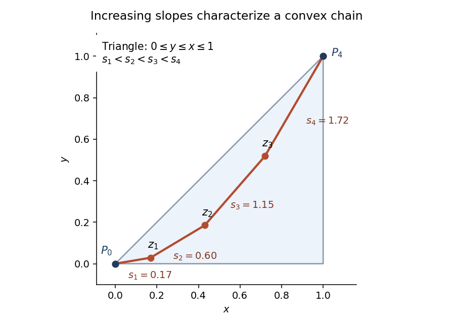
The volume for one specified label order is consequently $1/((k!{)}^2(k+1)!)$. There are $k!$ disjoint orders of the labels, and the joint uniform-triangle density is $2^k$. Hence the convex-chain probability in a triangle isFor example $p_1=1$ and $p_2=1/3$.

Let $C_k$ count the $k$-element subsets of the $n$ sampled points that are convex chains. By linearity of expectation, $\mathbb{E}{C}_k=\left(\genfrac{}{}{0ex}{}{n}{k}\right)p_k$. If $L_n\ge k$, an optimal chain contains a $k$-vertex subchain, since removing vertices from a convex polygon preserves convex position of the remaining vertices. Therefore, by the first moment method,We used $\left(\genfrac{}{}{0ex}{}{n}{k}\right)\le n^k/k!$, $(k+1)!\ge k!$, and $k!\ge (k/e{)}^k$, the last following from ${\sum }_{j=1}^k\log j\ge {\int }_1^k\log xdx$.

Take $k=\lceil 4e{n}^{1/3}\rceil$. If $k\le n$, the last bound is at most $32^{-k}<1/2$; if $k>n$, the event is empty. Every integer median $m_n$ must then satisfy $m_n<k$, and thereforeThe hint's curve $y=x^2$ is a parabola, not a hyperbola. The exact counting argument above proves the upper bound directly. The same chain probability is recorded in Ambrus and Bárány's analysis of longest convex chains.

Expand around the expectation $\mu$:Thus variance as the minimum mean squared error of a constant givesThe finite second moment also guarantees the finite first absolute moment needed below.

For a probability density function $f$, splitting at $a$ givesLet $F$ be the cumulative distribution function. Since a density gives no mass at a singleton, differentiating under this integral yields $H^{\prime }(a)=F(a)-(1-F(a))=2F(a)-1$. This derivative is nondecreasing, so $H$ is convex andThis is the median minimizes expected absolute loss property. The minimizer need not be unique: a gap in the density can give an interval of medians, all with the same loss.

The bounded classical solution is the heat-kernel convolutionThe two-dimensional heat kernel has integral one. Boundedness of $g$ permits differentiation under the integral for $t>0$, proving $u_t=\Delta u$ and $|u|\le \Vert g{\Vert }_{\infty }$. Its approximate identity property gives $u(x,t)\to g(x)$, locally uniformly since $g$ is continuous. This bounded solution satisfies the required Gaussian-growth bound.

For heat-equation uniqueness under Gaussian growth, let $w$ be the difference of two solutions, so $w(x,0)=0$ and $|w|\le M_0{e}^{a|x{|}^2}$ on a finite time interval. Choose $b>a$ and a slab $0\le t\le \tau <1/(4b)$. The positive comparison solutionsatisfies $({\Phi }_b{)}_t=\Delta {\Phi }_b$. For any $\epsilon >0$, its faster spatial growth makes $|w|\le \epsilon {\Phi }_b$ on a sufficiently large lateral cylinder boundary. At the initial boundary, $w=0$. The heat equation maximum principle applied to $\pm w-\epsilon {\Phi }_b$ proves the same inequality inside. First allow the cylinder radius to increase, then let $\epsilon \downarrow 0$. Repeating these slabs proves uniqueness on every finite interval with the stated uniform growth bound. No spatial integrability of $g$ is required.

At time $T$, this is Gaussian filtering with covariance $2TI$, hence $\sigma =\sqrt{2T}$ per coordinate. With the angular-frequency Fourier transform convention $\hat{f}(\xi )=\int e^{-ix\cdot \xi }f(x)dx$, the Gaussian filtering Fourier multiplier isFor merely bounded $g$, this identity is understood through tempered distributions. The multiplier leaves the zero frequency unchanged and attenuates large frequencies exponentially: it suppresses rapid noise fluctuations but blurs image edges. In cycles-per-length frequency $k$, the multiplier is $e^{-4{\pi }^{2}T|k{|}^2}$.

For the printed Perona-Malik equation, retain the supplied conductance $c(s)=s{e}^{-s^2/(2{\lambda }^2)}$, which includes an extra factor $s$. In one dimension write $p=u_x$ and $F(p)=c(|p|)p=p|p|e^{-p^2/(2{\lambda }^2)}$. Then $u_t=F^{\prime }(u_x)u_{xx}$, withThe forward-backward threshold for gradient-weighted exponential diffusion is thereforeAt $|u_x|=0$ and $\sqrt{2}\lambda$ the coefficient vanishes, giving degenerate diffusion. Increasing $\lambda$ increases the forward-diffusion range. Small nonzero slopes smooth, while large slopes formally sharpen; a negative coefficient produces short-wave growth and ill-posedness, so this is a dynamics explanation, not a general existence theorem for arbitrary data. Replacing the printed conductance by $e^{-s^2/(2{\lambda }^2)}$ would give threshold $\lambda$, but that is a different equation.

The four-neighbour mean expansion follows by Taylor expansion: opposing first and third derivatives cancel, soIf $u(x_0)={\mathrm{mean}}_h(u)(x_0)$ for every sufficiently small $h$, division by $h^2$ and passage to the limit give $\Delta u(x_0)=0$. This is a pointwise conclusion; it does not assert harmonicity in a whole neighbourhood.

For the area median over the disk, the disk-median curvature expansion, at a point where $|\nabla u|\ne 0$, isConsequently the analogous median fixed-point condition yieldsThis is the vanishing of the level-line curvature at $x_0$: to second order the level line is straight there. It need not be a straight segment. For example $u(x,y)=y+x^3$ has zero disk median at the origin for every radius, by odd symmetry, but its zero level line is the cubic $y=-x^3$. Vanishing curvature on an entire connected regular level arc would force that arc to be straight. The factor $1/6$ is for the disk's uniform area measure; a circle-boundary median has a different scale factor, while producing the same zero-curvature equation.

Put $Q(u)=\inf \{x\in \mathbb{R}:F(x)\ge u\}$ for $0<u<1$. This is the quantile function, rather than an ordinary inverse requiring strict increase. The limits of the distribution function at infinity make $Q(u)$ finite, and the fact that $F$ is a right-continuous function ensures $F(Q(u))\ge u$. ConsequentlyIncreasing $u$ shrinks the set in the infimum, so the quantile function is a monotone function. To prove the left continuity of the quantile function, fix $u$ and let $L={\sup }_{v<u}Q(v)\le Q(u)$. If $L<Q(u)$, choose $L<y<Q(u)$. Then $F(y)<u$, so some $v\in (F(y),u)$ satisfies $Q(v)>y$, a contradiction. Thus $Q(v)\uparrow Q(u)$ as $v\uparrow u$. At a flat stretch of the distribution function, the quantile function may jump immediately to the right, consistent with this left-continuous convention.

For the uniform order statistic, count the observations at most $u$. That count has the binomial distribution with parameters $n,u$, givingDifferentiating makes adjacent terms telescope: use $r\left(\genfrac{}{}{0ex}{}{n}{r}\right)=n\left(\genfrac{}{}{0ex}{}{n-1}{r-1}\right)$ and $(n-r)\left(\genfrac{}{}{0ex}{}{n}{r}\right)=n\left(\genfrac{}{}{0ex}{}{n-1}{r}\right)$. The probability density function is thereforeIn particular, $U_{(j)}$ has the Beta distribution with parameters $j,n-j+1$.

Write $m=Q(1/2)$ for the specified median. Continuity of the distribution function gives $F(m)=1/2$ and no mass at $m$, even if the distribution function has a flat stretch there. Thus $B={\sum }_i{1}_{\{X_i<m\}}$ has the binomial distribution with parameters $n,1/2$. Except on a null event, the order-statistic confidence interval for a median covers $m$ exactly when $j\le B\le n-j$. Symmetry of the binomial distribution makes its two failure probabilities equal. Alternatively, the probability integral transform givesHence the coverage is exactly $1-\alpha$, withThe asymmetric open/closed endpoint convention does not change the coverage because the continuous probability distribution assigns no mass to the median.

Write $f(x)=\mathrm{TS}\{x_1,\dots ,x_n\}$. Besides Talagrand's convex distance inequality, we use the precise squared edge bound for tours in the unit square stated above and the triangle inequality, which permits shortcutting a closed walk without increasing its length. We first prove the geometric comparison that connects these results.

For each fixed $x$, choose a cyclic tour $C$ with edge lengths ${\ell }_i$ satisfying ${\sum }_i{\ell }_i^2\le 4$. At vertex $x_i$, let $a_i(x)$ be the sum of the lengths of its two incident edges in $C$. The Cauchy-Schwarz inequality givesWe claim the weighted mismatch bound for Euclidean tours:To prove it, keep the vertices whose coordinates agree. In the cyclic ordering $C$, the deleted vertices split into consecutive runs between kept vertices. For one run, let $a,b$ denote its two boundary edge lengths and $S$ the sum of its internal edge lengths. Starting at the left kept endpoint, visit the run and return along the same path, at cost $2(a+S)$; starting at the right endpoint costs $2(b+S)$. Choose the cheaper detour. Its cost is at mostwhich is exactly the sum of $a_i(x)$ over that run. Attach these detours to a shortest tour through $y$, which already visits every kept point. The resulting closed walk visits all points of $x$; shortcut it using the triangle inequality. Summing the detour costs proves the claimed weighted mismatch bound for Euclidean tours. If there is just one kept vertex, the same argument uses that vertex as both endpoints of the unique run. If there are no kept vertices, $f(x)\le {\sum }_i{\ell }_i\le {\sum }_i{a}_i(x)$ proves the comparison directly. Repeated point locations cause no difficulty, since their connecting edges may have length zero.

Let $M$ be any median of $f(X)$ and set $A=\{y:f(y)\le M\}$. For $f(x)\ge M+t$, the weighted mismatch bound for Euclidean tours impliesThe weights have squared sum at most one, so $d_T(x,A)\ge t/4$. Since $\mathbb{P}(A)\ge 1/2$, Talagrand's convex distance inequality yieldsFor the lower tail, put $B=\{x:f(x)\le M-t\}$. If $\mathbb{P}(B)=0$ there is nothing to prove. For every $y$ with $f(y)\ge M$, apply the same weighted mismatch bound for Euclidean tours with its weights $a_i(y)$ and all $x\in B$. It gives $d_T(y,B)\ge t/4$. The set of such $y$ has probability at least $1/2$, so Talagrand's convex distance inequality instead givesCombining both tails,The bound has a constant fluctuation scale, independent of $n$. Only independence of the point coordinates and their support in the square are needed here; their uniform distribution was needed for the earlier lower bound on the expected value.

The useful form is Talagrand's convex distance inequality. Let $({\Omega }_i,{\mu }_i)$ be standard probability spaces, let $\Omega ={\prod }_{i=1}^n{\Omega }_i$ carry the product measure $\mu ={⨂}_i{\mu }_i$, and let $A\subset \Omega$ be a measurable event with $\mu (A)>0$. For $x\in \Omega$, form the mismatch vectorsThe Talagrand convex distance is the distance from zero to their closed convex hull:Equivalently, by the Hahn-Banach separation theorem for two convex sets,Nonnegative weights suffice because every mismatch vector has nonnegative coordinates. Talagrand's convex distance inequality statesIn particular, Markov's inequality gives the product-space concentration inequalityThe same conclusion is interpreted with outer probabilities if a distance set is not measurable; the continuous geometric function used below has measurable level sets. A median $M$ of a real random variable $Z$ means that $\mathbb{P}(Z\le M)\ge 1/2$ and $\mathbb{P}(Z\ge M)\ge 1/2$. Applying the displayed concentration inequality to suitable level sets will control deviations around a median.

For a nonnegative continuous event time, the survivor function is $F(t)=\mathbb{P}(T>t)$; here the printed $F$ denotes survival, not the usual cumulative distribution function. A lower median isFor a continuous strictly decreasing survivor function this is the unique solution of $F(m)=1/2$. If the curve has a flat stretch at $1/2$, the distribution has a nonunique median and the infimum specifies the lower endpoint.

The tail integral formula for moments follows from $T={\int }_0^{\infty }1\{T>t\}dt$ and Tonelli theorem. Therefore, when survival vanishes beyond $t^{\ast }$,If $F(t)>0$ at every finite time, the mean is finite precisely when ${\int }_0^{\infty }F(t)dt<\infty$. For a concrete sufficient condition, require $F(t)\le C{t}^{-1-\epsilon }$ for all $t\ge M>0$, with $C<\infty$ and $\epsilon >0$. The integral over $[0,M]$ is at most $M$, and the tail integral is at most $C{M}^{-\epsilon }/\epsilon$. An exponential tail bound also suffices. Merely having $F(t)\to 0$, or even $tF(t)\to 0$, does not suffice: a properly completed decreasing tail proportional to $1/(t\log t)$ for $t\ge e$ has infinite mean.

Let $a_1<a_2<\cdots$ be the distinct observed event times, $r_j$ the risk set size immediately before $a_j$, and $d_j$ the events there. Under independent censoring, the Kaplan–Meier estimator isIt starts at one, jumps down at events, and is unchanged by a pure censoring time; right censoring removes people from subsequent risk sets. If events and censorings coincide, the convention here processes events before censoring, so those censored at the recorded time are included just before the event. The estimated median is the first time the curve reaches or falls below $1/2$. If it never does during observation, the median is not estimable from the observed curve without tail assumptions.

With one remaining individual censored at $t_1$, no event factor is introduced. HenceThis is the terminal observed step value. With an empty risk set after $t_1$, continued horizontal plotting is a convention and supplies no information about the true later survivor function. The tail rests on one person and is imprecise; this is terminal censoring and survival-mean identifiability. If ${\varphi }_0>0$, the unrestricted mean cannot be obtained nonparametrically from this censored tail: extending the last positive step to infinity would give an infinite area, which does not establish an infinite population mean. A restricted mean survival time up to a suitably supported finite cutoff remains estimable.

Normalization of the probability density function givessoThe expected value isThe second moment isTherefore the variance is

For the median $m$,so

Expanding around the expected value $\mu$,because $\mathbb{E}[X-\mu ]=0$. Thereforewith equality exactly when $a=\mu$.

For the absolute loss,Leibniz differentiation gives, with $F(a)={\int }_{-\infty }^{a}f(x)dx$,Thus $H$ decreases while $F(a)<1/2$ and increases while $F(a)>1/2$. It is minimized at any median, characterized in the continuous case by

Let $m=F^{-1}(1/2)$ be the unique median. The influence function of the sample median isaway from $m$. Its second moment, equivalently the asymptotic distribution of a sample median, givesNo symmetry assumption is used: the density is evaluated at the actual median of $F$.

Choose a fixed $\alpha <1/2$. On the stated high-probability event, strictly more than half of the block means satisfy, simultaneously for every $\Vert v{\Vert }_2\le 1$,The median of a collection with a strict majority in an interval lies in that interval. Hence the same bound holds for $|{\mathrm{MOM}}_k(Xv)-{\mu }_0^{T}v|$ uniformly in $v$. Part b then giveswith probability at least $1-e^{-k/c_{\alpha }}$. Renaming the constant proves the claim.

Complementing every friendship sends every degree $d$ to $n-1-d$, and hence sends $S=M+L$ to $2(n-1)-S$. Since the random graph and its complement have the same law, the distribution of $S$ is symmetric about $n-1$, giving $\mathbb{E}S=n-1$.

The same symmetry gives equal probabilities strictly below and above $n-1$. There is positive probability at $n-1$: for odd $n$ use a regular graph of degree $(n-1)/2$; for even $n=2m$, use $K_{m,m}$ with a perfect matching removed and then restore one matching edge. Thus the lower median as defined is also $n-1$.

For this rate parametrization of the Laplace distribution, $\mu$ is its mean and median. By symmetry, $\mathbb{E}(X-\mu )=0$, while $|X-\mu |$ has exponential distribution with rate $\lambda$, soThe integral follows by two applications of integration by parts. The central limit theorem therefore givesWith known $\lambda$ and the supplied cutoff 2, an approximate 95% confidence interval isThis known-rate Laplace location confidence interval uses the sample mean; the later maximum-likelihood estimator of location need not be used to construct this valid asymptotic confidence interval.