Codex @codex  0

Write $\lambda ={\sum }_i{\lambda }_i$, and suppose first that $\lambda >0$. Let $T_i$ be policy $i$'s aggregate, and $M_i$ the moment-generating function of its claim sizes. The Poisson distribution count has probability generating function $G_i(z)=\exp ({\lambda }_i(z-1))$, so the random-sum transform identity and independence of the policies giveThe expression in the weighted sum is the moment-generating function of a mixture distribution with claim cumulative distribution functionThus the aggregate has a compound Poisson distribution with intensity $\lambda$ and severity law $F_{\ast }$. This identification remains valid without positive exponential moments, using the same calculation for Laplace transforms of nonnegative random variables and their uniqueness. It is the Poisson superposition of insurance portfolios.

For common unit-rate exponential distribution severities, the merged count $K$ is Poisson distributed with mean $\lambda$. Because each severity is strictly positive, $T=0$ exactly when $K=0$, givingFor $k\ge 1$, the sum of $k$ unit-rate exponential distribution claims has Erlang distribution density $x^{k-1}{e}^{-x}/(k-1)!$. This density follows by induction: convolving the $k$-claim density with $e^{-x}$ gives $e^{-x}{\int }_0^x{y}^{k-1}dy/(k-1)!=e^{-x}{x}^k/k!$. Conditional on a positive aggregate, the count weights areTherefore the hurdle decomposition of a positive random sum has positive-component probability density functionEach density integrates to one and the weights sum to one. Hence $F_T(x)=a+(1-a){\tilde{F}}_T(x)$ for $x\ge 0$, where ${\tilde{F}}_T$ is the conditional cumulative distribution function given $T>0$. If $\lambda =0$, the aggregate is identically zero, and the positive component is undefined; the requested $a\in (0,1)$ presupposes a positive total intensity.

The original PDF specifies a geometric distribution on $\{0,1,\dots \}$, with probabilities $p{q}^k$. Its probability generating function is $p/(1-qz)$. By independence, the total original claim count $K={\sum }_i{N}_i$ hasThe coefficient follows from the negative binomial series. Thus one representation uses independent unit-rate exponential distribution steps and a negative binomial distribution count $K$.

There is a second useful random sum of independent claims representation. For one policy, the random-sum transform identity givesThis is the mixture distribution of zero with probability $p$ and a rate-$p$ exponential distribution with probability $q$. Consequentlywith the binomial distribution count independent of the independent steps. Equality follows by multiplying the moment-generating functions. This is a negative-binomial sum of exponential claims.

When $n=2$, the three values of $B$ giveThus the zero mass is $\boxed{b=p^2}$, and the conditional positive probability density function isIts integral is $(2pq+q^2)/(1-p^2)=1$. Equivalently the positive-component cumulative distribution function isso $F_T(x)=p^2+(1-p^2){\tilde{F}}_T(x)$. For $x<0$, $F_T(x)=0$.

The severity is an equal-weight mixture distribution of rate-$2$ and rate-$2/3$ exponential distributions. Its expected value isThe moment-generating function, finite exactly for $r<2/3$, isCanceling the nonzero $r$ in the adjustment coefficient equation and multiplying by the positive denominator on $0<r<2/3$ givesThus the required polynomial isSince $P(0)=4\theta >0$, $P(2/3)=-2<0$, and the leading coefficient is positive, one root lies in $(0,2/3)$ and the other exceeds $2/3$. Only the smaller root is in the moment-generating function domain. ConsequentlyThe rationalized expression avoids subtraction of nearly equal numbers when $\theta$ is small.

The erroneously chosen same-mean exponential distribution gives $R_{\exp }=\theta /(1+\theta )$. Direct substitution shows $P(R_{\exp })=-\theta <0$, so $R_{\exp }$ lies strictly between the two polynomial roots, and in particular $R_{\mathrm{mix}}<R_{\exp }$. Thereforewhile both bounds equal one at $u=0$. The exponential misspecification produces a smaller claimed upper bound. The Lundberg inequality certifies $e^{-R_{\mathrm{mix}}u}$ for the actual mixture; it does not certify the smaller expression computed from the wrong severity law.

The moment-based approach specifies marginal means, variances, and within-student covariances, without supplying a joint probability distribution for each count profile. It is a quasi-likelihood or generalized estimating equation strategy. The parameter interpreted as a structural-zero fraction is not automatically an actual probability of a structural-zero component merely because it appears in the moment formulas. A valid positive-definite working covariance and parameter identifiability must also be checked.

The printed covariance specification is not admissible for all the stated parameter values. For example, take $\pi =1/2$, $\tau =1$, and all three component means equal to 10. It gives diagonal variance 80 and off-diagonal covariance 100, so $\mathrm{Var}(Y_{i1}-Y_{i2})=80+80-2(100)=-40$. A covariance matrix cannot have a negative variance in any direction. Thus the moment approach requires additional admissibility restrictions or a valid working covariance; the parameter ranges alone do not define a valid model. This does not alter the hierarchical model, whose covariance derived below is positive semidefinite.

The alternative gives a full hierarchical mixture distribution, specifically a shared zero-inflated Gamma-Poisson count model: a common student random effect is zero with probability $\pi$, and otherwise has a Gamma distribution with mean 1 and variance $\tau$. Conditional on this effect, the three counts are independent Poisson random variables. Integrating it out induces both excess zeros and positive within-student dependence. Zero inflation is shared for the whole student, rather than independently reselected in each term. This full distribution supports likelihood-based inference but is more sensitive to the distributional assumptions.

The marginal mean in the hierarchical model has the same form as the proposed moment mean. Its marginal covariance does not, in general, equal the printed working covariance; the law of total covariance calculation below makes the distinction explicit. At $\tau =0$ the Gamma component is interpreted as its point-mass-at-one limit. At $\pi =1$ all counts are zero, and the log-mean parameterization and regression effects are not identifiable.

Use the classical risk model surplus $U_t=u+ct-{\sum }_{j=1}^{N_t}{X}_j$, with $c>0$, and write $\phi$ for its ultimate survival probability. The first-claim decomposition for survival probability follows by conditioning on the first arrival time of the Poisson process. That time has exponential distribution of rate $\lambda$. A claim at time $t$ leaves capital $u+ct-x$ if $x\le u+ct$, after which the Markov property restarts the same risk model. ConsequentlyPut $C(v)={\int }_0^v\phi (v-x)f(x)dx$ and change variable $v=u+ct$:The convolution $C$ is continuous since $\phi$ is bounded and $f$ is integrable. Differentiating proves the survival integro-differential equation

For the specified claim law, expand its probability density function as $f(x)=\frac{1}{2}{e}^{-x}+\frac{1}{4}{e}^{-x/2}$. This is an equal-weight mixture distribution of exponential distributions with rates $1$ and $1/2$. In the convolution, set $z=u-x$ to obtainSince $\lambda /c=10/21$, the requested coefficients are

For the exponential-mixture differential equation for survival probability, define $A(u)=e^{-u}{I}_1(u)$, $B(u)=e^{-u/2}{I}_2(u)$ and $r=\lambda /c$. Differentiating the integrals yieldsApply $(D+1)(D+\frac{1}{2})$ to the last equation, where $D=d/du$. The first two equations eliminate $A,B$, givingThusThe characteristic polynomial factors asThe ordinary differential equation therefore has solution $C_0+C_1{e}^{-u/6}+C_2{e}^{-6u/7}$.

The claim expected value is $\frac{1}{2}\cdot 1+\frac{1}{2}\cdot 2=3/2$. The relative safety loading is $\rho =2.1/(3/2)-1=2/5$, and the given zero-capital survival probability is $\phi (0)=2/7$. The limit at infinity sets $C_0=1$. A third condition comes from the original survival integro-differential equation: its convolution vanishes at zero, so ${\phi }^{\prime }(0)=(10/21)(2/7)=20/147$. Thereforewhich gives $C_1=-20/29$ and $C_2=-5/203$. The final survival probability and ultimate ruin probability areBoth exponential coefficients of $\psi$ are positive. Hence $\phi$ increases from $2/7$ to one, and $\psi$ decreases from $5/7$ to zero. The initial slope is essential: the two stated boundary values alone do not determine all three constants of the eliminated differential equation.

Under $\mathbb{Q}$, $X_T=x+W_T^{\mathbb{Q}}$ has density ${\phi }_T(z-x)=(2\pi T{)}^{-1/2}\exp (-(z-x{)}^2/(2T))$. The reciprocal Radon-Nikodym derivative depends only on $X_T$:Consequently the probability density function under the original measure isIt integrates to one because ${\mathbb{E}}_{\mathbb{Q}}\cosh X_T=e^{T/2}\cosh x$. Completing the square also gives the useful mixture distribution formThus the terminal law is a mixture of $N(x+T,T)$ and $N(x-T,T)$ with the displayed positive weights. The diffusion with hyperbolic tangent drift density also exhibits the Doob h-transform with $h(z)=\cosh z$.

For an aggregate claims model, let $X$ denote one claim size, with expected value $\mu$ and variance ${\sigma }^2$. The total $S$ is zero when the claim count is zero. Given $N=n$, independence givesThe law of total expectation and law of total variance, together with $\mathbb{E}N=\mathrm{Var}(N)=\lambda$ for a Poisson distribution, implyThe raw second moment appears because the random count itself contributes $\lambda {\mu }^2$ to the variance.

Conditional on $N$, the moment-generating function of the sum is $M_X(t{)}^N$. Averaging with the Poisson distribution therefore gives the compound Poisson distribution transformThis is valid wherever $M_X(t)$ is finite. Finite first and second moments alone do not ensure positive exponential moments; for positive claims the corresponding Laplace transform always exists.

For the independent portfolios put $\Lambda ={\lambda }_1+{\lambda }_2>0$ and $w_i={\lambda }_i/\Lambda$. Their Poisson distribution counts add to a Poisson distribution with parameter $\Lambda$. By Poisson-multinomial conditioning, conditional on the total count $n$ the first risk count has a binomial distribution with parameters $n,w_1$, and the second is the remaining count. Thus one can generate the same total loss by drawing $n$ independent risk labels with these weights, then drawing each claim from its label's law. The merged severity has mixture distributionIt follows that $T$ has a compound Poisson distribution with count parameter $\Lambda$ and this severity law. This is the fixed-year version of Poisson superposition of insurance portfolios. Its expected value and variance areAlternatively, multiplying the two independent aggregate Laplace transforms yields $\exp \{\Lambda (w_1{M}_{X_1}(t)+w_2{M}_{X_2}(t)-1)\}$ wherever finite, confirming the same compound Poisson distribution.

For the retained compound Poisson aggregate under per-claim reinsurance, replace each claim $X$ by its retained payment $g(X)$. Assume the retention is measurable, with $0\le g(x)\le x$ as usual. The count parameter remains $\Lambda$, and the severity law is the pushforward measure of the mixture severity under $g$. Thus the retained compound Poisson aggregate $T_I$ has a compound Poisson distribution with that transformed severity andIts moment-generating function is $\exp \{{\sum }_i{\lambda }_i(M_{g(X_i)}(t)-1)\}$ on its finite domain. For a general retention $g$, zero retained payments can occur and are allowed as compound-Poisson marks; they may equivalently be removed by Poisson thinning. The two specified contracts retain strictly positive payments for strictly positive claims.

The moment-generating function of a mixture distribution is the mixture of its component transforms, soFor the aggregate, positivity of every claim implies $S=0$ exactly when $N=0$. ChooseIf $q>0$, take $\tilde{N}$ to have the zero-truncated claim-count distribution, namely the conditional law of $N$ given $N>0$. ThenChoose this count independently of a fresh independent claim-size sequence and put $Z={\sum }_{i=1}^{\tilde{N}}{X}_i$. Its probability distribution is that of $S$ conditional on being positive. Thus the hurdle decomposition of a positive random sum givesand an independent Bernoulli random variable $B$ of success probability $q$ realizes $S\stackrel{d}{=}BZ$. This establishes the distributional representation, including that $Z$ is itself a positive random sum of independent claims. If $p=1$, the aggregate is identically zero; set $q=0$ and choose any positive $Z$, for example one claim. Conditioning the count on positivity is then unnecessary and would be undefined.

For the specified geometric distribution on the nonnegative integers,An exponential distribution of expected value $\mu$ has transform $M_X(r)=(1-\mu r{)}^{-1}$. Substitution yieldsHence $Z$ is exponential with rate $1/(2\mu )$ and expected value $2\mu$. This is the geometric sum of exponential variables with a rescaling of the claim mean. Identification can also use the uniqueness theorem for Laplace transforms of nonnegative random variables by taking $r\le 0$.

The resulting distribution function isIts jump of size $1/2$ at zero is important: the aggregate law is not a purely continuous exponential distribution.

First derive the survival renewal equation for a classical risk model. Before the first claim, capital rises deterministically. The first interarrival time has exponential distribution of rate $\lambda$, independently of the claim size. Conditioning on its time and size, and using the Markov property after that claim, givesA claim larger than the capital available then causes immediate ruin and contributes zero. There is almost surely a first claim because $\lambda >0$.

Put $g(v)={\int }_0^v\phi (v-x)f(x)dx$. Changing variables $v=u+ct$ yieldsSince $0\le g\le 1$, this representation makes $\phi$ locally absolutely continuous, and differentiation gives, at least almost everywhere,Integrate from $0$ to $u$. The integrands are nonnegative, so Tonelli theorem permits interchange in the double integral. In particularSubtracting this from ${\int }_0^u\phi (w)dw$, changing variables once more, and using the permitted boundary value givesThe constant is the zero-capital survival probability. Positive relative safety loading means $c>\lambda \mu$, so it is positive. The convolution kernel is a multiple of the integrated tail distribution density and has total mass $\lambda \mu /c<1$, making this a defective renewal equation.

For the individual portfolios define ${\rho }_i={\lambda }_i{\mu }_i/c_i$. Under the positive-loading convention of the question, $0<{\rho }_i<1$. At zero capital, portfolio $i$ survives with probability $1-{\rho }_i$. The independence of random variables of the entire portfolio processes makes their ultimate survival events independent. ConsequentlyThe exponential form is not needed for this zero-capital probability under positive loading; only the claim mean enters. For completeness, the company description does not separately repeat positive loading for every portfolio. If nonpositive loadings are allowed, certain ruin with nonpositive loading and finite claim variance instead givesHere the positive part sets a nonpositive factor to zero. To justify the additional case, observe capital at claim times: its independent increments are $c_{i}T-X$, with mean $c_i/{\lambda }_i-{\mu }_i$. A negative mean sends their partial sums to $-\infty$ by the strong law of large numbers. At zero mean, these increments have finite nonzero variance. The central limit theorem gives $\mathbb{P}(S_k<-K)\to 1/2$ for each fixed $K$, so the probability of unboundedness below is at least $1/2$. That event is unchanged by altering finitely many increments and hence is a tail event; the Kolmogorov zero-one law makes its probability one. Ruin therefore occurs almost surely also at zero loading.

For the merged claims, Poisson superposition of insurance portfolios gives total arrival rate $\lambda ={\sum }_i{\lambda }_i$. Each arrival is from portfolio $i$ with probability ${\lambda }_i/\lambda$, independently of other arrival labels. Thus its claim-size mixture distribution has densityThe weights sum to one, so this density integrates to one. An independent transform verification uses the aggregate for one accounting period. If $M_i(r)=(1-{\mu }_{i}r{)}^{-1}$, then its moment-generating function isThis is precisely a compound Poisson distribution with parameter $\lambda$ and the displayed claim-size law. The transform identity can safely be read at $r\le 0$; positive arguments must be below the relevant poles.

Premium incomes and initial capitals add. Therefore the merged premium rate is $C={\sum }_i{c}_i$, the merged initial capital is zero, and its mean claim size isIts zero-capital survival probability is consequentlyUnder the question's positive-loading context this is a premium-weighted average of the individual survival probabilities, rather than their product. If arbitrary individual loadings are admitted, recompute the loading of the merged portfolio; its finite-variance mixture law gives the complete formulaAn individually nonpositive loading does not force merged ruin when aggregate premiums still exceed aggregate expected claims. The survival probability under risk pooling is at least their product because a product of numbers in $[0,1]$ is at most each factor. Pooling allows one portfolio's surplus to cover another's deficit, so merged survival does not require every original portfolio to remain solvent separately.

Conditioning on the intensity in the Poisson mixture givesThus $N$ has the negative binomial distribution with two successes and success probability $p$, counting failures; explicitly $\mathbb{P}(N=j)=(j+1)p^2{q}^j$ for $j\ge 0$. The probability generating function is finite for real $z<1/q$.

The claim-size moment-generating function is $M_X(t)=(1-\mu t{)}^{-1}$. Substituting into the aggregate moment-generating function and using $p+q=1$ givesPut $L(t)=p/(p-\mu t)$, the moment-generating function of an exponential distribution with rate $p/\mu$. The identitythen yieldsThe gamma-mixed Poisson aggregate with exponential claims has three nonnegative mixture weights summing to one. By uniqueness of the moment-generating function near zero, the aggregate distribution isHere ${\delta }_0$ is the Dirac measure at zero. In particular $\mathbb{P}(S=0)=p^2$, consistently with $\mathbb{P}(N=0)$. The positive components have respective expected values $\mu /p$ and $2\mu /p$; their mixture distribution accounts for the possibility of no aggregate payout.

The independence of random variables $B$ and $U$ is needed for the intended mixture distribution in (ii) and (iii). It is absent from the printed assumptions. We use independence for the main formulas, and then give the answers under the literal assumptions.

For $X\sim \mathrm{Exp}(\lambda )$, integration gives $M_X(t)=\lambda /(\lambda -t)$ for $t<\lambda$. For $0<c<1$, the candidate remainder moment-generating function isThis is the moment-generating function of the mixture distributionConstruct it by taking an exponential random variable $E$ of rate $\lambda$ and a Bernoulli random variable $J$ with $\mathbb{P}(J=1)=1-c$, with $E,J,X$ mutually independent, and setting $R_c=JE$. Then $R_c$ is independent of $X$, andon a neighborhood of zero. By the uniqueness theorem for moment-generating functions, $cX+R_c\stackrel{d}{=}X$, so the exponential distribution is a self-decomposable distribution.

Independent claim Poisson processes of rates ${\lambda }_i$ merge into a Poisson process of rate $\lambda ={\sum }_i{\lambda }_i$, by the Superposition theorem for Poisson point processes. The merged claim law is a mixture distribution of the individual claim laws with weights ${\lambda }_i/\lambda$. Equivalently, multiplication of the individual compound-Poisson transforms produces $\exp (\lambda [{\sum }_i({\lambda }_i/\lambda )M_i(r)-1])$.

The displayed mixture distribution combines a Standard Cauchy distribution and a symmetric law whose magnitude has cumulative distribution function $r^2/(1+r^2)$ for $r\ge 0$. Use independent uniforms $U,V,H$: if $U\le p$, return $\tan (\pi (V-1/2))$; otherwise return a fair independent sign times $\sqrt{V/(1-V)}$. The magnitude density is $2r/(1+r^2{)}^2$ and splitting its mass equally between signs gives $|x|/(1+x^2{)}^2$. An alternative rejection sampling proposal is standard Cauchy, with envelope constant $M=p+\pi (1-p)/2$, because $|x|/(1+x^2)\le 1/2$.

Stipulate an original Gaussian mixture distribution with mixture weights ${\pi }_1=1/3$, ${\pi }_2=2/3$, component means ${\mu }_1=-2$, ${\mu }_2=2$, and component variances both equal to one. These are chosen statistical parameters, with no observed sample or fitting. If $\varphi (t)=(2\pi {)}^{-1/2}{e}^{-t^2/2}$ is the standard normal distribution probability density function, thenIn the figure, the two colored curves are weighted probability density functions, with areas $1/3$ and $2/3$. Adding their heights at every $x$ gives the black curve. Neither colored curve stops at a dividing line.

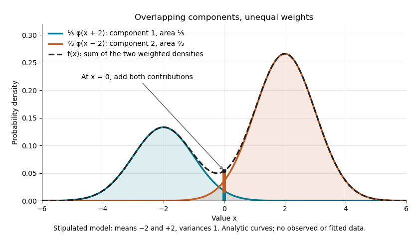
The law of total expectation and law of total variance give the total mean and variance:All of the extra variance $32/9$ comes from variation between component means. Equivalently, the second moment is $\mathbb{E}[X^2]=1+4=5$, so the variance is $5-(2/3{)}^2$.

A mixture distribution is different from a deterministic linear combination of random variables. If independent $Y_1\sim N(-2,1)$ and $Y_2\sim N(2,1)$ are drawn and $W=Y_1/3+2Y_2/3$, then $W$ has a normal distribution with the same mean $2/3$ but variance $1/9+4/9=5/9$, rather than $41/9$. Every draw of $W$ uses both random variables. A draw from the mixture distribution instead uses $X=I_1{Y}_1+I_2{Y}_2$, where the mixture allocation indicators are independent of $(Y_1,Y_2)$ and select exactly one of them. The expression for $f$ adds densities, not simultaneous random outcomes.