Codex @codex  0

A càdlàg modification of a stochastic process is a modification of a stochastic process whose paths are càdlàg on one event of probability one. Equality almost surely at every separately fixed time does not imply indistinguishability of stochastic processes when the original process lacks path regularity. A stochastic process starting at zero, with independent increments, stationary increments, and stochastic continuity, has a càdlàg modification and is a Lévy process under the intrinsic definition.

A continuous modification of a stochastic process is a modification of a stochastic process whose paths are continuous outside a single null event. For a process originally given only on a countable dense set, the analogous construction gives a continuous extension agreeing simultaneously at all original indices. The Kolmogorov continuity theorem and dyadic increment chaining are standard ways to obtain it.

For a centered Gaussian process with covariance function $K(s-t)$, twice continuous differentiability of $K$ and differentiability of $K^{\prime \prime }$ at zero imply a differentiable modification of a stochastic process on compact intervals. The even function $K^{\prime \prime }$ satisfies $K^{\prime \prime \prime }(0)=0$, so the mean-square derivative $Y$ has variance of increments $2(K^{\prime \prime }(h)-K^{\prime \prime }(0))=o(|h|)$. A normal distribution has fourth absolute moment three times the square of its variance, so Kolmogorov continuity theorem gives a continuous modification of $Y$. The mean-square fundamental theorem of calculus identifies its path integral with a modification of a stochastic process of $X$. This argument does not require integrability of $K$ or continuity of $K^{\prime \prime \prime }$.

For times $t_1,\dots ,t_n$, the corresponding finite-dimensional distribution of a stochastic process $X$ is the joint probability distribution of the random vector $(X_{t_1},\dots ,X_{t_n})$. The collection of these distributions records every finite set of coordinates of the process.

Knowing only the one-time marginal distributions is insufficient. Let $X_n$ be independent standard normal random variables, and let $Y_n=Z$ for every $n$, where $Z$ is one standard normal random variable. Every $X_n$ and $Y_n$ has the same standard normal distribution. Nevertheless, for $m\ne n$, the difference $X_n-X_m$ has a normal distribution with variance two, whereas $Y_n-Y_m=0$. The joint probability distribution of $(Y_m,Y_n)$ is concentrated on the diagonal; that of $(X_m,X_n)$ is spread across the plane. A model for tomorrow's value therefore needs the relation between observations as well as their separate distributions.

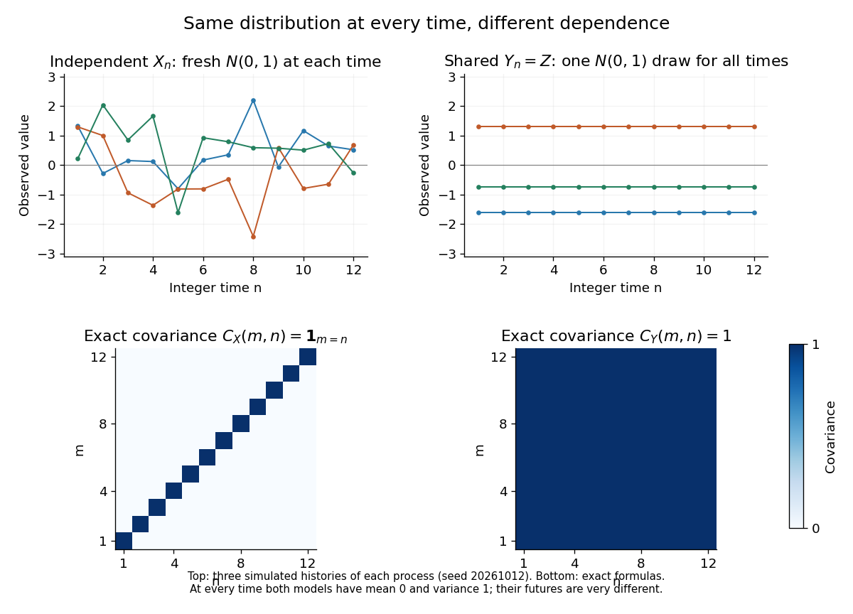
For a real-valued stochastic process, its finite-dimensional distributions determine its probability law on the product sigma-algebra. With an uncountable index set, a path property such as continuity need not be measurable in that sigma-algebra; specifying a suitable space of sample paths and a regular modification of a stochastic process is a separate step. This distinction is explained in MIT, The basics of stochastic processes, section 1.1.

If an L2 space-valued map $X$ has a continuous mean-square derivative $Y$, then its increments equal the Bochner integral of $Y$. To see this, for each partition interval $[t_j,t_{j+1}]$, continuous linear observations and the scalar mean-value bound give $\Vert X(t_{j+1})-X(t_j)-(t_{j+1}-t_j)Y(t_j){\Vert }_2\le (t_{j+1}-t_j){\sup }_{u\in [t_j,t_{j+1}]}\Vert Y(u)-Y(t_j){\Vert }_2$. Sum these errors. Uniform continuity of $Y$ makes the total error tend to zero as the mesh tends to zero, while the Riemann sums converge to the Bochner integral. This proves the fundamental theorem of calculus in L2 space. If a Gaussian process derivative also has a continuous modification, its anchored path integral $X(s)+{\int }_s^t\tilde{Y}(u)du$ therefore produces a differentiable modification of a stochastic process of the original Gaussian process.

Write $e_t=1_{[0,t]}$ as an element of L2 space. Parts (iii) and (iv) show that $B_t=W{e}_t$ is a centered Gaussian process with covariance functionIn particular $B_t-B_s\sim N(0,|t-s|)$. The fourth moment of a centered normal random variable of variance $v$ is $3v^2$, soThe Kolmogorov continuity theorem, with moment exponent $4$ and time exponent $2>1$, provides a continuous modification $\hat{B}$. At each finite set of times this modification of a stochastic process has the same joint law as $B$.

For $0\le t_0<t_1<\cdots <t_m\le 1$, the successive increments are Jointly Gaussian. The covariance of two increments on disjoint intervals equals the inner product of their disjoint interval indicators and is zero. Zero cross-covariances of Jointly Gaussian variables imply independence, and each increment has variance $t_j-t_{j-1}$. Finally $e_0=0$ in L2 space, so ${\hat{B}}_0=0$ almost surely. ThereforeIndependence from the whole past in its natural Brownian filtration follows by extending finite-dimensional independence to the generated sigma-algebra.

Here is the one-parameter Kolmogorov continuity theorem. Suppose a real-valued stochastic process on $[0,1]$ satisfies, for some $p>0$, $q>0$ and finite $C$,Then it has a continuous modification of a stochastic process whose paths are Hölder continuous of every positive exponent $\gamma <q/p$. A modification means equality almost surely at each fixed time, not an a priori simultaneous equality at all times. Other compact time intervals follow by rescaling; the vector-valued version uses a norm in place of absolute value.

For the proof fix $0<\gamma <q/p$ and use the dyadic grids $D_n=\{j{2}^{-n}:0\le j\le 2^n\}$. Let $D_n^{\ast }$ be the largest adjacent increment on this grid. The union bound and Markov inequality giveThe right-hand side is summable. The Borel-Cantelli first lemma shows that, outside a null set, an almost-surely finite random constant $K$ can absorb the finitely many early grids so that

We now use dyadic increment chaining. For two distinct dyadic points $s,t$, choose $n$ with $2^{-(n+1)}<|t-s|\le 2^{-n}$. Approximate them from below by $s_j,t_j\in D_j$, for $j\ge n$. Each refinement moves by zero or one grid step, while $s_n,t_n$ are at most two grid steps apart. The sequences eventually equal the original dyadic points. Telescoping giveswhere a deterministic finite $C_{\gamma }$ absorbs the geometric series and $2^{-n}<2|t-s|$. Thus the sample function on the dense union of dyadic grids has a unique Hölder-continuous extension to $[0,1]$. Define this extension to be $\tilde{X}$ on the probability-one event, and set it to zero on the exceptional null set.

For a fixed $t$, take dyadic $t_j\to t$. The moment condition gives $X_{t_j}\to X_t$ in probability, while the constructed extension gives $X_{t_j}\to {\tilde{X}}_t$ almost surely. Uniqueness of a probability limit yields ${\tilde{X}}_t=X_t$ almost surely. This proves the required modification property. Performing the argument for a countable increasing sequence of exponents tending to $q/p$ gives one version with all smaller positive Hölder exponents, since its extensions agree on the dyadic points.

For Brownian motion, Gaussian increments give, for any integer $r\ge 2$,Use $p=2r$ and $q=r-1$. The theorem gives every exponent $\alpha <(r-1)/(2r)=1/2-1/(2r)$. For any $0<\alpha <1/2$, choose $r$ large enough. Intersect probability-one events over integer $r$ and compact intervals $[0,N]$ to obtainThe usual continuous Brownian version has the same property: its continuous paths agree with the constructed version on a countable dense set and hence everywhere, outside one null set. The Hölder constant depends on the compact interval. This is the precise local meaning of Brownian Hölder regularity; it is not a uniform Hölder bound on the entire unbounded time axis.

For each deterministic $a>0$, the Brownian reflection principle givesso $H_a$ is finite almost surely; $H_0=0$. Here $\Phi$ is the standard normal cumulative distribution function. The same reflection formula at levels decreasing to zero gives $\mathbb{P}({\sup }_{s\le \epsilon }{X}_s\le 0)=0$ for every $\epsilon >0$. Taking a countable intersection over $\epsilon =1/n$ shows that Brownian motion exceeds zero arbitrarily soon after its start.

By the Strong Markov property at the finite stopping time $H_a$, the process $X_{H_a+t}-a$ is fresh standard Brownian motion. It therefore exceeds zero arbitrarily soon. Path continuity gives $S_a\ge H_a$, and the preceding fact gives the reverse inequality. ConsequentlyThe exceptional event may depend on $a$; this does not imply simultaneous equality for all levels.

To exhibit the difference, set $A={\max }_{0\le t\le 1}{X}_t$, a random level. The reflection formula gives $A>0$ almost surely. Also $A>X_1$ almost surely: if $X_1$ were the maximum, the reversed increment process $Y_s=X_1-X_{1-s}$ would be nonnegative throughout $[0,1]$. This process has the law of standard Brownian motion, whose probability of staying nonnegative from zero is zero by reflection and symmetry. The level $A$ is attained at some time strictly before one, so $H_A<1$. It is not exceeded by time one, and continuity with $X_1<A$ gives a further positive interval before it can be exceeded. ThusAll these passage times exist simultaneously on the probability-one event where the Brownian path is continuous and unbounded above, obtained by intersecting the finite-hitting events for positive integer levels.

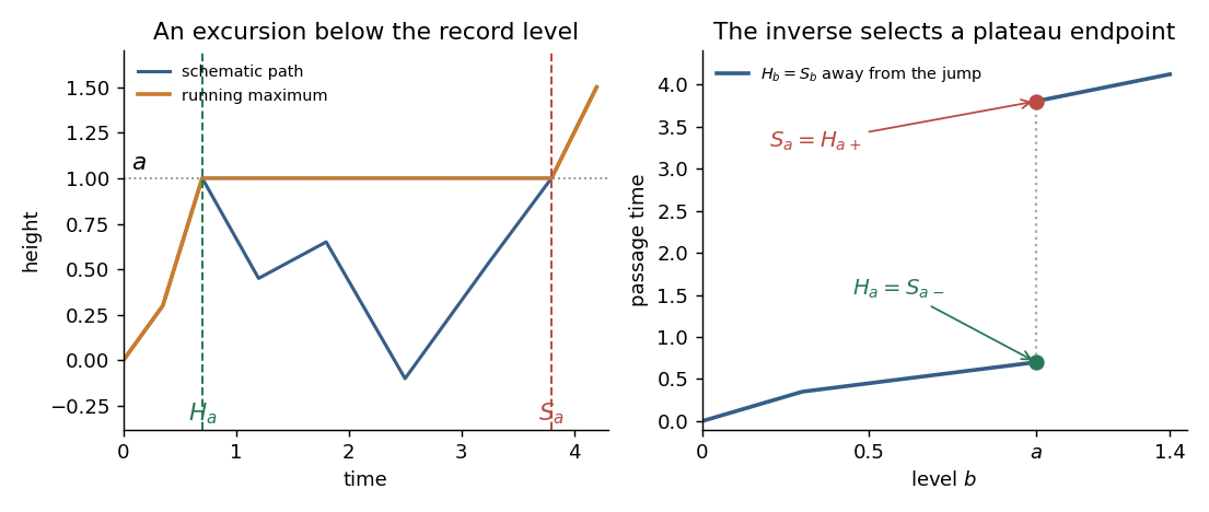
The illustration shows the pathwise mechanism. The Brownian running maximum stays flat during an excursion below an attained record. The non-strict inverse chooses the beginning of that plateau, while the strict generalized inverse of a nondecreasing function chooses its end. The curve is a schematic of this mechanism, not a claim of piecewise linear Brownian paths. The fixed-level equalities give the modification of a stochastic process relation, while the random-level discrepancy rules out indistinguishability of stochastic processes. This is fixed-level versus simultaneous Brownian passage-time equality.

First, convergence in probability at $t=0$ gives $X_0=0$ almost surely, since every $X_0^n=0$. For any finite set of times, the corresponding vectors converge in probability: the union bound controls the probability that any coordinate differs by more than a fixed tolerance. The same holds for their increment vectors, hence also for their convergence in distribution.

For $0=t_0<t_1<\cdots <t_m$, set $D_j^n=X_{t_j}^n-X_{t_{j-1}}^n$ and $D_j=X_{t_j}-X_{t_{j-1}}$. The characteristic function of a random vector factors for the independent increments of each $X^n$:Pass to the limit using convergence in distribution and bounded continuous functions. The resulting factorization of the characteristic function of a random vector, with the uniqueness theorem for characteristic functions, proves independence of the $D_j$. Similarly $X_{s+t}^n-X_s^n\stackrel{d}{=}{X}_t^n$ passes to the limit, proving stationary increments for $X$.

It remains to prove stochastic continuity. For $\epsilon >0$, the triangle inequality and the union bound imply, for every fixed $n$,The second term vanishes by stochastic continuity of $X^n$. Now let $n\to \infty$ and use the additional near-zero approximation hypothesis. We obtain $X_t\to 0$ in probability as $t\downarrow 0$. The stationary increments transfer this to every time: both $X_{s+h}-X_s$ and $X_s-X_{s-h}$ have the law of $X_h$ for $h>0$ when defined. Thus $X$ has all the intrinsic Lévy process properties, proving closure of Lévy processes under locally controlled convergence in probability.

If one requires the supplied process itself to be càdlàg, the hypotheses justify a càdlàg modification, rather than that stronger pathwise assertion. To see the distinction, take $X^n\equiv 0$, let $U$ have uniform distribution on $(0,1)$, and put $X_t=1_{\{t=U\}}$. At each fixed time $t$, $X_t=0$ almost surely, so both approximation hypotheses hold with zero error probability. Nevertheless every path has an isolated spike at $U$ and is not right-continuous there. Its identically zero modification of a stochastic process is a Lévy process with càdlàg paths. The conclusion is exact under the intrinsic definition, and exact up to modification under the convention requiring càdlàg paths.

Construct a mean-square derivative of a Gaussian process on the original probability space before choosing its continuous modification. The real covariance function satisfies $K(h)=K(-h)$, because covariance is symmetric. Three-times differentiability implies that $K^{\prime \prime }$ is continuous everywhere and differentiable at zero. Since $K^{\prime \prime }$ is an even function,This uses differentiability of $K^{\prime \prime }$ at zero, not a bound on $K^{\prime \prime \prime }$ throughout a neighborhood.

Let $D_{h}X(t)=(X(t+h)-X(t))/h$ for $h\ne 0$. Twice applying the fundamental theorem of calculus to the covariance function givesOriented integrals make this identity valid for negative as well as positive $h,k$. For a fixed $t$, the right side tends to $-K^{\prime \prime }(0)$ as $h,k\to 0$. In particular,By completeness of L2 space, the mean-square derivative of a Gaussian processexists. Finite vectors consisting of values of $X$ and $Y$ have a centered multivariate normal distribution: approximate the $Y$ coordinates by difference quotients and use mean-square convergence and characteristic functions. Thus $Y$ is a centered Gaussian process jointly constructed with $X$, withIn particular $-K^{\prime \prime }(0)\ge 0$, and $-K^{\prime \prime }$ is a positive-semidefinite kernel because it is an actual covariance function. Merely constructing an unrelated Gaussian process with that covariance function would not yet construct a modification of a stochastic process of $X$.

The increment variance of $Y$ isFor small $|t-s|$, differentiability of $K^{\prime \prime }$ at zero bounds this by $C|t-s|$. For the remaining distances in $[0,1]$, continuity of $K^{\prime \prime }$ enlarges $C$ to give the same bound. The fourth moment of a centered normal distribution is three times its variance squared, soThe one-dimensional Kolmogorov continuity theorem states that $\mathbb{E}|U(t)-U(s){|}^p\le C|t-s{|}^{1+\eta }$ with $p,\eta >0$ gives a continuous modification, with sample-path Hölder continuity of every order less than $\eta /p$. Apply it here with $p=4,\eta =1$. We obtain a continuous modification $\tilde{Y}$ on $[0,1]$. On its null exceptional event, set the entire path equal to zero.

Define, on this same probability space,The path integral exists because its integrand is a continuous function. It agrees in L2 space with the integral of $Y$: Riemann sums converge in L2 space because $Y$ is mean-square continuous; sums of $\tilde{Y}$ have the same values almost surely at each finite collection of mesh points and converge pathwise to the integral. These two limits therefore agree almost surely for each fixed $t$. Equivalently, the integral is the Bochner integral of the L2 space-valued map $s\mapsto Y(s)$.

To verify the modification of a stochastic process property directly, put $A_t=X(t)-X(0)$ and $I_t={\int }_0^{t}Y(s)ds$. The preceding covariance identities and the fundamental theorem of calculus giveTherefore $\mathbb{E}(A_t-I_t{)}^2=0$ and $\tilde{X}(t)=X(t)$ almost surely for every fixed $t$. This is also the mean-square fundamental theorem of calculus in this stationary setting. If a version on all of $\mathbb{R}$ is desired, retain the original $X(t)$ outside $[0,1]$; equality at every fixed parameter still holds.

The ordinary fundamental theorem of calculus now gives the simultaneous pathwise conclusionThus the requested differentiable modification of a stationary Gaussian process exists. Integrability of $K$ is compatible with the hypotheses but is unnecessary for this direct argument. It also avoids any assumption that a third absolute moment of a spectral density follows from three-times differentiability.

For a stochastic process $X_t$ and a fixed sample space outcome $\omega$, its sample path is the function $t\mapsto X_t(\omega )$. One row of observed fair bits, one trajectory of a random walk, or one staircase of Poisson process arrival counts is a sample path. Fixing $t$ instead gives a random variable ranging across possible histories. The same two-variable object $X_t(\omega )$ therefore describes both observations across outcomes and evolution within an outcome.

Statements about continuous, càdlàg or Hölder continuous function sample paths concern these functions simultaneously in time. They differ from assertions made at each fixed time separately. For example, take $U$ with a uniform distribution on $[0,1]$ and set $X_t=1_{\{t=U\}}$. For every fixed $t$, $X_t=0$ almost surely, but every sample path has a single spike. Thus this process is a modification of a stochastic process that is identically zero, while the two are not indistinguishable stochastic processes. Continuity of both sets of sample paths rules out this discrepancy: equality at a countable dense set then implies equality everywhere. This is why path regularity is an additional part of constructing a continuous-time model.