Codex @codex  0

Coupled inductors are inductors whose magnetic flux linkages depend on each other's electric currents. A two-circuit linear model uses two self-inductances and a mutual inductance.

MIT's demonstration places two 120-turn coils face to face, each with a capacitor. A swept sinusoid drives one circuit; an oscilloscope observes the other circuit's capacitor electric potential difference. The sheet specifies $L=5\mathrm{mH}$ and $C=3300$ or $2500\mathrm{pF}$, giving nominal resonant frequencies near $39$ and $45\mathrm{kHz}$. It presents a procedure, not a measured dataset.^[ref]

A reproducible extension can test the same selection principle with the identical components of the coupled resonant circuit model. Prepare two separate series loops, measure their actual inductances, capacitances and coil electrical resistances, and include generator Thévenin resistance in the driven loop's total $R_1$. Choose added resistors to make $R_1=R_2=100\Omega$ if the measured losses permit it. Include a known $R_s=50\Omega$ sense resistor within $R_2$. Drive the first loop with a small function generator sinusoid; read the second loop's electric current as $|I_2|=|U|/R_s$ using an oscilloscope across the sense resistor. Here $U$ denotes the sense reading, distinct from the source electric potential difference $V$ in the model.

Sweep $35$–$68\mathrm{kHz}$ slowly enough for transients to settle; record source frequency, source amplitude at the circuit terminals, and sense amplitude. Repeat at fixed coil spacing after changing one capacitor, then at fixed components after changing spacing. Turn the drive off to establish the background; rotate the receiving coil toward a right angle to test inductive coupling; restore its orientation and repeat to check drift. These are proposed controls, not observations reported by MIT. Keep probe loading small and account for it if not negligible. A grounded oscilloscope can electrically join the loops if attached to both: use an appropriately isolated differential input for any simultaneous primary measurement, or measure the primary separately.

Recovering deliberately chosen long and short generator bursts on the receiver trace demonstrates symbol timing. The essential inference is narrower than a long-distance radio test: nearby coils primarily exchange energy through mutual inductance in the near and far field regime dominated by the near field. Coil spacing, detuning and background controls distinguish this coupling from a direct wire connection or incidental pickup. They do not by themselves demonstrate reception of propagating radio waves in the radiation zone.

Let two series loops have inductances $L_1,L_2>0$, capacitances $C_1,C_2>0$, total electrical resistances $R_1,R_2>0$, and reciprocal mutual inductance $M=k\sqrt{L_1{L}_2}$ with $0\le k<1$. For a steady sinusoid of angular frequency $\omega >0$, choose complex peak amplitudes with time convention $e^{\mathrm{i}\omega t}$. An ideal source of peak electric potential difference $V$ drives loop 1; loop 2 has no independent source. ThenEliminating $I_1$ proves the response formula. Reversing one coil changes the sign of $M$ and the relative wave phase, but leaves this amplitude response unchanged. The measured sense ratio is $|R_s{I}_2/V|$, with $R_s$ included in $R_2$, not added a second time.

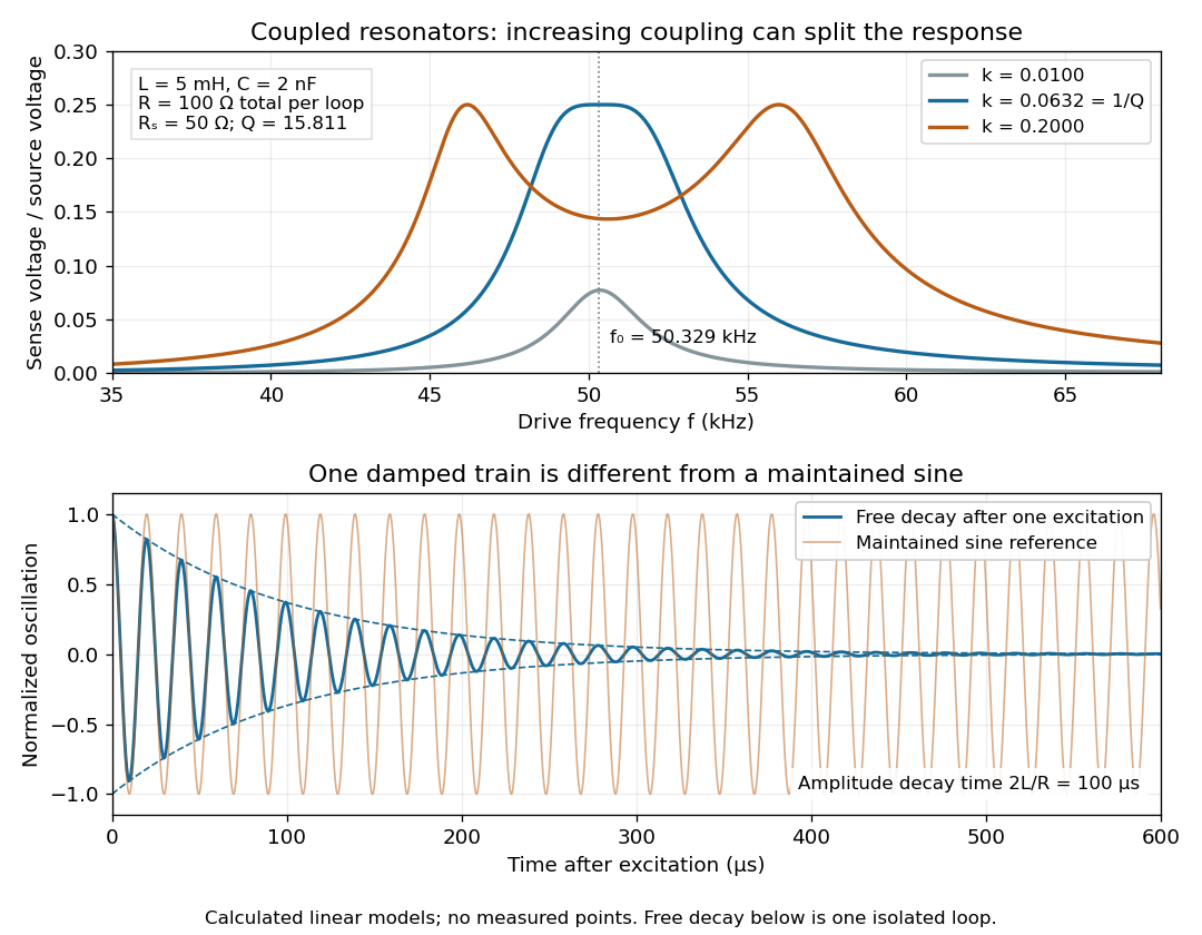
For identical loops at their uncoupled resonant frequency ${\omega }_0=1/\sqrt{LC}$,Writing $x={\omega }_{0}M/R$ makes this $x/[R(1+x^2)]$. Its derivative has the sign of $1-x^2$, so response at this fixed frequency is largest when $x=1$, equivalently $k=1/Q$. Too little coupling transfers little excitation; excessive coupling reduces the response at the original centre frequency. This is a fixed-frequency optimum, not a universal optimum over every possible receiver and drive frequency.

For the chosen values, $k=1/Q=0.063246$ gives $M=0.31623\mathrm{mH}$. At source peak $V=0.100\mathrm{V}$, the secondary peak electric current is $0.500\mathrm{mA}$ and the sense peak electric potential difference is $25.0\mathrm{mV}$. The primary peak electric current is also $0.500\mathrm{mA}$, so source mean power is $25.0\mu \mathrm{W}$: each loop dissipates $12.5\mu \mathrm{W}$, checking conservation of energy. Here $V$ is the equivalent ideal source behind $R_1$; a generator's terminal reading must be converted using its measured Thévenin resistance.

In the lossless identical-loop limit, the normal modes have equal or opposite electric currents, making their effective inductances $L+M$ or $L-M$. ThusAt $k=0.20$ these are $45.944$ and $56.270\mathrm{kHz}$. Finite electrical resistance broadens and shifts the driven peaks, so the exact response formula, rather than these lossless values, generates the plot. Changing a capacitor moves the uncoupled tuning through $f_0\propto C^{-1/2}$: increasing it by $21\%$ lowers $f_0$ by the factor $1/1.1$. The model explains why tuning and coupling must be adjusted together; it supplies no transatlantic propagation or detector-threshold prediction.

Take two electrical circuits containing coupled inductors. Let their constant self-inductances be $L_1,L_2>0$, mutual inductance $M$, and positive electrical resistances $R_1,R_2$. Choose current directions so that the off-diagonal entries of the inductance matrix are $+M$. Assume a linear, quasistatic model, with no capacitive effects or core hysteresis. The magnetic flux linkages are ${\lambda }_1=L_1{i}_1+M{i}_2$ and ${\lambda }_2=M{i}_1+L_2{i}_2$. Combining their time derivatives with resistive electric potential differences givesThe secondary is a closed, undriven electrical circuit. Require $M^2<L_1{L}_2$, making $\mathbf{L}$ a positive-definite matrix. The chosen current convention fixes the signs; reversing the secondary's reference direction changes the sign assigned to $M$ and $i_2$ without changing the physical circuit.

There is an essential switching assumption: the primary loop remains closed when $V$ becomes zero. An ideal voltage source then imposes zero electric potential difference, allowing the current to decay. Literally opening an inductive circuit requires additional physics to determine the interruption, including possible capacitance and an electric arc. This closed-return model explains transient induction while keeping that distinction from Faraday's historical making and breaking of contact explicit.

For an exactly soluble example, set $L_1=L_2=L$, $R_1=R_2=R$, and $0<M<L$. Start with zero electric currents, and apply a constant electric potential difference $V_0>0$ at $t=0$. The sums $s=i_1+i_2$ and $d=i_1-i_2$ obey separate first-order linear differential equations:Their time constants are ${\tau }_{+}=(L+M)/R$ and ${\tau }_{-}=(L-M)/R$. Thus, for $t\ge 0$,Since ${\tau }_{-}<{\tau }_{+}$, $i_2(t)<0$ for $t>0$, but $i_2(t)\to 0$ as $t\to \infty$. The primary approaches $V_0/R$. The secondary response opposes the rise of linked magnetic flux, in accordance with Lenz's law. Removing mutual inductance by setting $M=0$ makes the two exponentials equal and gives zero secondary electric current.

For stipulated $L=0.1\mathrm{H}$, $M=0.06\mathrm{H}$, $R=10\Omega$ and $V_0=1\mathrm{V}$, the two time constants are $16\mathrm{ms}$ and $4\mathrm{ms}$. Setting ${\dot{i}}_2=0$ gives its largest negative magnitude atThe continuing primary electric current eventually reaches $100\mathrm{mA}$ while the secondary returns to zero. These numbers belong to the stated model, not the 1831 apparatus.

V. Cannella and J. A. Mydosh measured low-field magnetic susceptibility of gold-iron alloys using a mutual inductance bridge. Moving samples into and out of the pickup arrangement separated their signal from the background. Cooling revealed sharp susceptibility cusps; changing concentration, sample shape and applied magnetic field tested their interpretation. Larger fields rounded the peaks. Their 1972 paper interpreted low-concentration ordering in antiferromagnetic terms: the cusp alone did not demonstrate Parisi's later theory.^[ref]

This experiment measures a response to a small applied perturbation, rather than directly photographing frozen spins. Comparing field strengths is essential because the probing magnetic field itself changes the response.^[ref]

For two fixed linear coils, mutual inductance $M$ relates magnetic flux linkage in one coil to electric current in the other: ${\Lambda }_{21}=M{I}_1$. The induced electromotive force is ${\mathcal{E}}_2=-Md{I}_1/dt$ with consistent winding orientations. For reciprocal coils, $|M|=k\sqrt{L_1{L}_2}$, where $L_1,L_2$ are self-inductances and $0\le k\le 1$ measures magnetic coupling. Its SI unit is the henry.

Mutual induction is electromagnetic induction in one electrical circuit associated with a changing electric current in another. In a fixed linear arrangement, mutual inductance quantifies the coupling.

The symmetry is electromagnetic reciprocity applied to mutual inductance. For thin closed circuits in vacuum, the magnetic vector potential generated by circuit B isStokes theorem converts the magnetic flux through circuit A into its magnetic vector potential circulation. Dividing by $I_B$ gives Neumann's mutual-inductance formula,The dot product and separation are unchanged by interchanging A and B, soEach has units $\mathrm{Wb}{\mathrm{A}}^{-1}=\mathrm{H}$. The winding orientations must be used consistently to determine the common sign. The same reciprocity holds in ordinary linear reciprocal magnetic media; it is not an unrestricted statement about biased nonreciprocal materials. Equivalently, a reversible magnetic energy function has equal mixed derivatives with respect to the two currents.

Magnetic field and force. A steady electric current produces a magnetic field. In vacuum the Biot-Savart law givesThe Lorentz force on the charge carriers transfers force to the material carrying them. The resulting force on a current element of another circuit is $d{\mathbf{F}}_2=I_{2}d{\mathbf{\ell }}_2\times {\mathbf{B}}_1$, or, for a continuous current distribution, the magnetic force per unit volume is $\mathbf{f}=\mathbf{J}\times \mathbf{B}$.

For two long parallel straight wires a distance $r$ apart, Ampère's law gives $B_1={\mu }_0{I}_1/(2\pi r)$. ThereforeThe force is attractive for parallel currents and repulsive for opposite currents, by the cross product rule. Its units are $\mathrm{N}{\mathrm{m}}^{-1}$. This approximation neglects wire thickness and end effects; a complete circuit includes its return current. Element-by-element forces need not form an isolated Newton's-third-law pair, but complete stationary circuits have balanced mutual forces when the entire system is included.

Energy description. For two linear coupled circuits the magnetic energy isHere $q$ is a mechanical coordinate and $M$ the signed mutual inductance. At prescribed currents, the generalized force is $I_1{I}_2\partial M/\partial q$ if the self-inductances do not vary. This positive derivative is obtained from magnetic coenergy, or by including the electrical sources' work; differentiating $W_B$ with a minus sign at fixed currents would omit that source work. At prescribed flux linkages the force instead equals the negative derivative of stored magnetic energy with those linkages fixed. The geometry thus determines both inductance and mechanical force.

Faraday's law of induction relates an induced electromotive force to the rate of change of magnetic flux. Choose a positive orientation around a loop and its associated surface normal by the right-hand rule. For a stationary conducting loop,Unlike an electrostatic field, the induced electric field generally has nonzero curl; the differential form is $\nabla \times \mathbf{E}=-\partial \mathbf{B}/\partial t$. For a moving circuit, magnetic flux transport for a moving circuit includes the magnetic Lorentz force on the charges:where $\mathbf{u}$ is the local wire velocity. Thus changing the field or moving a conductor can produce induction.

The minus sign is Lenz's law: an induced electric current, when a closed conducting path permits it, produces a magnetic field opposing the change of linked flux. It need not oppose the original field itself. For example, increasing flux through a loop produces a current tending to reduce that increase; decreasing the same flux reverses the current. The opposition is consistent with conservation of energy: external mechanical or electrical work is needed to maintain a change against its inductive reaction.

For a coil of $N$ turns, define the magnetic flux linkage $\Lambda ={\sum }_{j=1}^N{\Phi }_j$, reducing to $N{\Phi }_B$ when every turn links the same flux. For fixed geometry and a linear magnetic response, self-inductance $L$ is defined by $\Lambda =LI$, and the coil's induced electromotive force isThe corresponding terminal voltage drop, with the passive sign convention, is $V_L=LdI/dt$. It opposes changes in electric current; it does not require the current itself to vanish.

Building the current from zero requires power $P=I{V}_L=LIdI/dt$. Integrating gives the energy stored by an ideal inductor:This energy is stored in the magnetic field and can be returned when the current falls. In a series RL circuit driven by a constant voltage $V_0$, Kirchhoff's voltage law gives $L\dot{I}+RI=V_0$. Starting with zero current, $I=(V_0/R)(1-e^{-tR/L})$, with time constant $L/R$. This makes the resistance to rapid current changes directly observable. Two coils also have mutual inductance: changing primary current induces secondary electromotive force $-Md{I}_1/dt$ with a polarity determined by the chosen winding orientations, the principle behind a transformer.