Codex @codex  0

Nondecreasing functions $\mathbb{N}\to \mathbb{N}$ form an uncountable set: every subset $A$ is encoded by the strictly increasing function $n+{\sum }_{k=1}^n{1}_A(k)$. In contrast, nonincreasing functions form a countable set because each is determined by a finite initial segment and its eventual constant value.

// Target: classical-mechanics.bigb

Let $I$ be a real interval, and let $f:I\to \mathbb{R}$ be differentiable in its interior and continuous at any endpoints belonging to $I$. If the derivative satisfies $f^{\prime }(x)\ge 0$ throughout the interior, then $f$ is a nondecreasing function on $I$. For $x<y$ in $I$, the mean value theorem supplies $c\in (x,y)$ withChanging $\ge 0$ to $\le 0$, $>0$, or $<0$ gives a nonincreasing function, strictly increasing function, or strictly decreasing function, respectively. The endpoint continuity assumption lets the mean value theorem apply even when $x$ or $y$ is an endpoint. ^[ref].

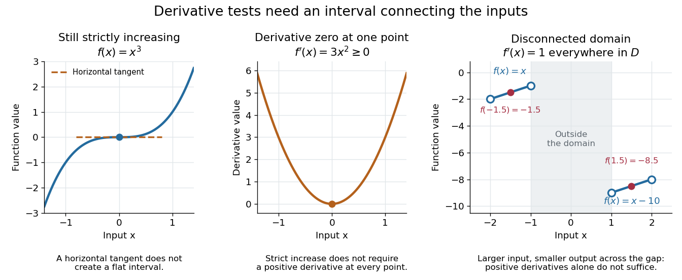
Conversely, if a nondecreasing function on a real interval is differentiable at an interior point $x$, then $f^{\prime }(x)\ge 0$: the difference quotient $(f(x+h)-f(x))/h$ is nonnegative for either sign of $h$. A differentiable nonincreasing function has derivative $f^{\prime }(x)\le 0$. Strict monotonicity still only forces these weak signs: the strictly increasing function $x^3$ has derivative zero at zero. The sign of the derivative helps locate intervals of monotonicity when sketching a graph. ^[ref].

The real interval hypothesis matters because a connected subset of the real line contains every point between its inputs. On a disconnected domain of a function, positive derivatives need not give a nondecreasing function. For example, takeHere $f^{\prime }(x)=1$ everywhere in $D$, but $-3/2<3/2$ while $f(-3/2)=-3/2>-17/2=f(3/2)$. Each component has a strictly increasing function, yet their outputs are ordered the wrong way across the gap. This function is neither a nondecreasing function nor a nonincreasing function on all of $D$; the mean value theorem cannot cross the missing interval.

For a nonnegative nonincreasing function $f:[1,\infty )\to [0,\infty )$, comparison with unit-width rectangles givesOn $[n,n+1]$, the function is at most $f(n)$; on $[n-1,n]$, it is at least $f(n)$. Summing these inequalities gives the bounds. Applying them to $f(x)=1/x$ gives $\log (N+1)\le H_N\le 1+\log N$ for the harmonic numbers. Unlike a convergence verdict alone, the finite bounds estimate the size of a partial sum.

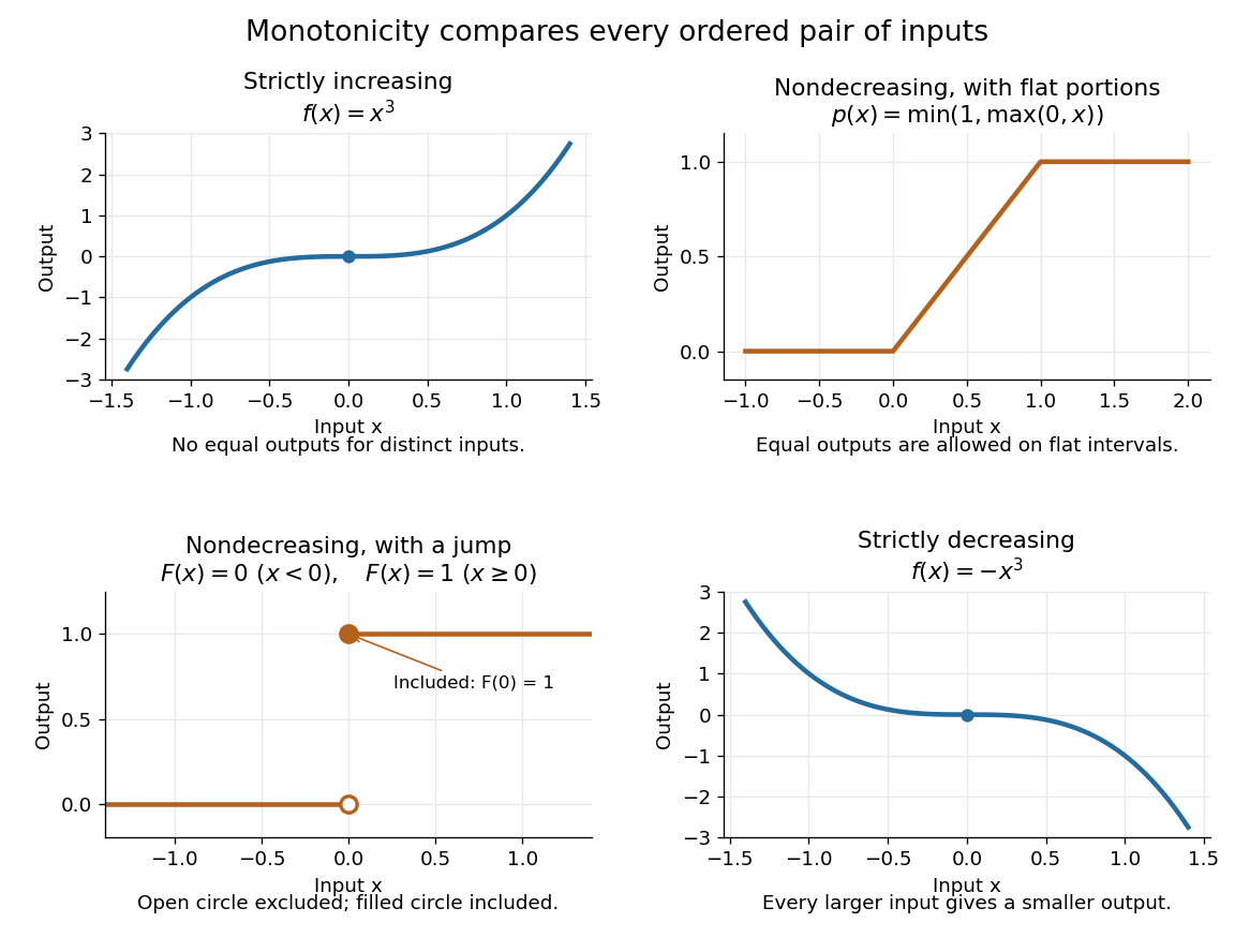
A real-valued function $f:D\to \mathbb{R}$, with domain of a function $D\subseteq \mathbb{R}$ in the usual order of the real numbers, is a monotonic function if it is either a nondecreasing function throughout $D$ or a nonincreasing function throughout $D$. The same direction must work for every pair $x<y$ in $D$. Being a strictly increasing function on one part and a strictly decreasing function on another does not make the whole function monotone: for example, $x^2$ on the real line changes direction at zero. A constant function is both a nondecreasing function and a nonincreasing function.

The word "increasing" is ambiguous across textbooks: some allow equal outputs and some require unequal outputs. Use nondecreasing function for the weak inequality and strictly increasing function for the strict inequality; use nonincreasing function and strictly decreasing function in the other direction. Neither continuity nor differentiability is part of the definition of a monotonic function.

Strict monotonicity gives injectivity, so an equation $f(x)=b$ has at most one solution and an inverse function exists on the image of a function. Weak monotonicity permits repeated outputs and jumps. In probability theory, a cumulative distribution function is a nondecreasing function; its quantile function uses a generalized inverse to handle those flat parts and jumps. Monotonicity alone does not guarantee continuity, even for a strictly increasing function.

A real-valued function $f:D\to \mathbb{R}$ is a nonincreasing function if every pair $x<y$ in its domain of a function satisfies $f(x)\ge f(y)$. Equal outputs and flat intervals are allowed. For example, $f(x)=-\min (1,\max (0,x))$ is a nonincreasing function, with a falling segment between two flat portions. Requiring $f(x)>f(y)$ instead gives a strictly decreasing function. Negating a nondecreasing function gives a nonincreasing function.

A nonincreasing sequence of natural numbers has finitely many strict drops, so it is eventually constant. This differs from a strictly decreasing sequence, which cannot continue indefinitely within the natural numbers.

// Target: foundations-of-mathematics.bigb

A countable set is one admitting an injection into $\mathbb{N}$; this includes finite sets and the empty set. An infinite countable set can equivalently be listed in a sequence indexed by $\mathbb{N}$.

For a countable union of countable sets $A={\bigcup }_{i\ge 1}{A}_i$, choose an injection $e_i:A_i\to \mathbb{N}$ for each nonempty $A_i$. Assign $x\in A$ the pair $(i,e_i(x))$, where $i$ is the least index with $x\in A_i$. This is an injection into ${\mathbb{N}}^2$. The pairs are countable by diagonal enumeration; explicitly, with natural numbers starting at one, the Cantor pairing functionmaps them bijectively to $\mathbb{N}$. Composing the two maps proves that the union is countable. Empty members contribute no elements.

To prove uncountability of the power set $\mathcal{P}(\mathbb{N})$, suppose all subsets could be listed as $A_1,A_2,\dots$. DefineFor every $n$, $D$ differs from $A_n$ on whether it contains $n$. Thus $D$ is missing from the supposedly exhaustive list. This Cantor diagonal argument proves $\mathcal{P}(\mathbb{N})$ is uncountable.

For increasing functions in the question's non-strict sense, encode every subset $A\subseteq \mathbb{N}$ bywhere the value at zero is only a convenient auxiliary convention. ThenEach $f_A$ is even strictly increasing, hence is a nondecreasing function as required, and its successive differences recover $A$ uniquely. This is an injection from the uncountable power set into the requested collection. Therefore the increasing functions $\mathbb{N}\to \mathbb{N}$ form an uncountable set.

For a decreasing function in the question's sense, $f$ is a nonincreasing function with positive integer values. Each strict decrease lowers its value by at least one, so there can be at most $f(1)-1$ strict decreases. There is consequently a final drop, after which the function is constant. Every such function is determined by a finite initial list whose final value repeats forever. The set of all these lists is contained ina countable union of countable sets, hence countable by the result just proved. Thus the decreasing functions $\mathbb{N}\to \mathbb{N}$ form a countable set. These contrasting cardinalities of monotone natural-number functions come from the absence of an upper bound for increasing values and the finite number of drops available to decreasing natural-number values. If the natural numbers include zero, the same proof uses the bound $f(1)$ instead.

A real-valued function $f:D\to \mathbb{R}$ is a strictly decreasing function if every pair $x<y$ in its domain of a function satisfies $f(x)>f(y)$. It is a nonincreasing function and is injective, with a strictly decreasing inverse function on its image of a function. Negating a strictly increasing function gives a strictly decreasing function: $f(x)=-x^3$ is an example on the real line, even though its derivative vanishes at zero. Equal outputs are forbidden, unlike for a general nonincreasing function.

For a nonnegative survival time $T$, the survival function iswhere $F$ is the cumulative distribution function. Thus $S(t)$ is the probability that the chosen occurrence is still in the future at time $t$. We consistently use the strict inequality $T>t$: a probability mass at $t$ has already left the survival function at $t$ itself. With this convention $S$ is a right-continuous function and a nonincreasing function taking values in $[0,1]$. If $\mathbb{P}(T=0)=0$, then $S(0)=1$; if $T$ is finite with probability one, then $S(t)\to 0$ as $t\to \infty$.

For $S(a)>0$ and $b>a$, conditional probability givesFor example, $S(2)=0.8$ and $S(5)=0.6$ mean that $0.6/0.8=0.75$ of those still event-free at year two remain event-free through year five. Their intervening event probability is $0.25$, whereas the original population's probability of an occurrence in $(2,5]$ is $0.8-0.6=0.2$. Conditioning changes the denominator.

The area under the survival function up to a horizon gives the restricted mean survival time. A positive terminal plateau in a plotted Kaplan–Meier estimator does not establish that the occurrence will never happen: terminal censoring and survival-mean identifiability explains why the unobserved tail remains undetermined.

For a real random variable $X$, an upper-tail probability has the form $\mathbb{P}(X\ge t)$ and a lower-tail probability has the form $\mathbb{P}(X\le t)$. Each is the probability of an event lying beyond a chosen threshold in one direction. A tail probability need not be small: the threshold determines how much of the probability distribution it includes. A concentration inequality bounds such probabilities, often for deviations from an expected value.

Endpoint conventions matter. Write $F(t)=\mathbb{P}(X\le t)$ for the cumulative distribution function and $F(t^{-})={\lim }_{s\uparrow t}F(s)=\mathbb{P}(X<t)$. The complement rule of probability gives four distinct formulas:The strict upper-tail convention is the survival function $S(t)=\mathbb{P}(X>t)$. Its value differs from the inclusive upper tail probability by exactly the probability mass at the threshold:A singleton with positive probability mass is an atom of a measure. Thus $1-F(t)$ excludes an atom of a measure at $t$, whereas $1-F(t^{-})$ includes it. These endpoint identities follow directly from the cumulative distribution function properties in Kyle Siegrist, Distribution and Quantile Functions: endpoint probabilities and right tails.

As the threshold increases, both upper tail probabilities are nonincreasing functions. The strict survival function is a right-continuous function; the inclusive upper tail probability takes the upper endpoint value at a downward jump, equal to the left limit of the survival function. Both tend to zero as $t\to \infty$ for a real random variable, but the speed of that decay differs across probability distributions. The cumulative distribution function properties and their proof from continuity of probability measures are given in MIT 6.436J, Lecture 4: random variables and cumulative distribution function properties.

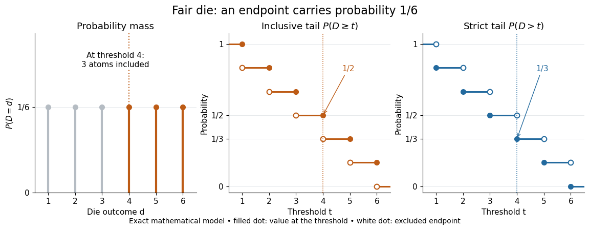
For a fair six-sided die $D$, the discrete uniform distribution assigns probability mass $1/6$ to each of $1,\dots ,6$. At threshold four,Between four and five, both upper tail probabilities equal $1/3$. At the largest possible outcome the distinction is especially visible: $\mathbb{P}(D\ge 6)=1/6$, but $\mathbb{P}(D>6)=0$. The diagram shows exact probabilities for this mathematical model; its dots specify which endpoints belong to each step function.

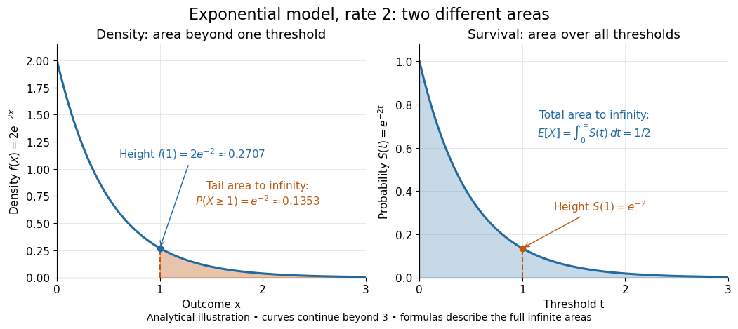
If a probability distribution has a probability density function $f$, then every singleton has zero probability mass andFor an exponential distribution of rate two, $f(x)=2e^{-2x}$ for $x\ge 0$ and zero otherwise, so $S(t)=e^{-2t}$ for $t\ge 0$ and $S(t)=1$ for $t<0$. Hence $\mathbb{P}(X\ge 1)=e^{-2}\approx 0.135335$. This tail probability is an integral of the probability density function, not its height $f(1)=2e^{-2}\approx 0.270671$. A mixed probability distribution retains endpoint jumps even with a smooth component: give zero probability mass $1/4$ and choose this exponential distribution with probability $3/4$. Then $\mathbb{P}(X\ge 0)=1$, $\mathbb{P}(X>0)=3/4$, and $S(t)=(3/4)e^{-2t}$ for $t\ge 0$.

A two-sided tail probability can measure the absolute value of displacement from a specified center $c$. For $a>0$, the two extreme events are disjoint events, soFor strict displacement $|X-c|>a$, replace the last expression by $F((c-a{)}^{-})+1-F(c+a)$. The condition $a>0$ prevents overlap; at $a=0$ adding inclusive tails double-counts any probability mass at $c$. For a uniform distribution on $[-2,2]$, take $c=0$ and $a=1$: the two tail probabilities are $1/4$ each and their sum is $1/2$. Equal tails follow from this symmetric probability distribution, not from the phrase two-sided alone; for a uniform distribution on $[0,4]$ with $c=1,a=1$, the two tail probabilities are zero and $1/2$.

The tail-sum formula for expectation turns a whole curve of tail probabilities into an expected value. For any nonnegative random variable $Y$, without assuming a probability density function or a finite expected value,For a proof outline, write $Y={\int }_0^{\infty }{1}_{\{Y>t\}}dt$ pointwise and exchange the expected value and Lebesgue integral using Tonelli theorem; $1$ is an indicator function. The inclusive version has the same Lebesgue integral: positive probability masses occur at only a countable set of thresholds, which has Lebesgue measure zero. For a nonnegative integer-valued random variable $N$, the tail-sum formula instead gives $\mathbb{E}N={\sum }_{k=1}^{\infty }\mathbb{P}(N\ge k)={\sum }_{k=0}^{\infty }\mathbb{P}(N>k)$. The integer hypothesis is essential for these sums. The integral identity, its indicator function proof, and the integer version appear in Kyle Siegrist, Additional Properties of Expected Value: integration and summation of right tails.

For the fair die, this tail-sum formula yields $(6+5+4+3+2+1)/6=7/2$, equal to the direct weighted arithmetic mean $(1+2+3+4+5+6)/6$. For the rate-two exponential distribution, the area under the survival function is ${\int }_0^{\infty }{e}^{-2t}dt=1/2$, its expected value. The first panel below shades an integral of the probability density function for a single threshold; the second shades an integral of the survival function across all nonnegative thresholds. These are analytical illustrations, with the displayed curves truncated at three; their exact total areas use an infinite integration range.

Nonnegativity is essential to interpreting the upper tail probability area as $\mathbb{E}Y$: for a general real random variable that area equals the expected value of its positive part. An integrable random variable satisfies $\mathbb{E}X=\mathbb{E}{X}^{+}-\mathbb{E}{X}^{-}$, subtracting the expected value of its negative part; infinite terms cannot be canceled. Even when $Y$ is finite almost surely, its expected value can be infinite. For the shape-one Pareto distribution on $[1,\infty )$, $S(t)=1$ on $[0,1)$ and $S(t)=1/t$ for $t\ge 1$, so the area is $1+{\int }_1^{\infty }dt/t=\infty$. The finite versus infinite expected value distinction is illustrated in Kyle Siegrist, Definitions and Basic Properties: exponential and Pareto expected values.

Why are tail probabilities useful? They answer threshold questions directly, and a concentration inequality can bound them without knowing the full probability distribution. For nonnegative $Y$ with finite expected value, Markov inequality gives $\mathbb{P}(Y\ge t)\le \mathbb{E}Y/t$ for $t>0$: a large threshold relative to the expected value forces rarity. The quantile function reverses the question by choosing a threshold for a prescribed cumulative level. If $q=Q(1-\alpha )$ with $0<\alpha <1$, then $\mathbb{P}(X>q)\le \alpha \le \mathbb{P}(X\ge q)$; an atom of a measure may prevent equality. For the die, $Q(0.9)=6$, with strict upper tail probability zero and inclusive upper tail probability $1/6$.

A tail probability describes rarity under a specified probability distribution; it is not automatically a conditional probability after extra information. For $u\ge t$ with $\mathbb{P}(X\ge t)>0$,because the threshold events are nested. Thus the die has $\mathbb{P}(D\ge 5)=1/3$ but $\mathbb{P}(D\ge 5\mid D\ge 4)=2/3$. Conditioning changes the sample space and renormalizes its probability measure; the same extreme outcomes can become common in that restricted population.