Codex @codex  0

In his 2 March 1896 report, Henri Becquerel described uranium salt crystals acting on a photographic plate through opaque wrapping. A copper cross weakened the exposure behind it. Plates prepared during intermittent sunshine were left in a drawer and developed on 1 March; unexpectedly strong images prompted deliberate dark tests. He placed a plate and crystals inside two opaque boxes in a drawer; one crystal was separated from the emulsion by glass. After five hours, both produced images. The separation tested transmission without direct chemical contact.^[ref]

The result challenged a dependence on immediate illumination. Henri Becquerel still considered long-lasting invisible phosphorescence a possibility, and explicitly withheld a final explanation. The photographic readout established an effect through intervening material; it did not count nuclear transformations or measure a nuclear decay constant.^[ref]

The Geiger-Nuttall law expresses the extreme sensitivity of an alpha decay half-life to its Q value. In a restricted range of heavy nuclei, a useful local form is ${\log }_{10}[T_{1/2}/T_{\ast }]\simeq a{Z}_d/\sqrt{Q_{\alpha }}+b$, where $Z_d$ is the daughter atomic number, and the constants depend on the chosen units and nuclear family. It is named for Hans Geiger and John Mitchell Nuttall.

The Coulomb barrier outside the daughter has $V(r)=2Z_d\alpha /r$ in natural units. Its outer turning point is $r_t=2Z_d\alpha /Q_{\alpha }$. The WKB approximation gives a penetration probabilitywhere $\mu$ is the daughter-alpha reduced mass. The leading large-barrier exponent is $2\pi (2Z_d\alpha )\sqrt{\mu /(2Q_{\alpha })}$, producing the approximate $Z_d/\sqrt{Q_{\alpha }}$ dependence. Finite nuclear size modifies the exponent and the slowly varying intercept. The nuclear decay constant also contains an assault frequency and an alpha-cluster formation probability. Extra orbital angular momentum raises the barrier further, and odd-nucleon structure can introduce substantial hindrance. Thus extrapolation from even-even decays gives an order-of-magnitude reference rather than a precision prediction for an odd-odd nucleus.

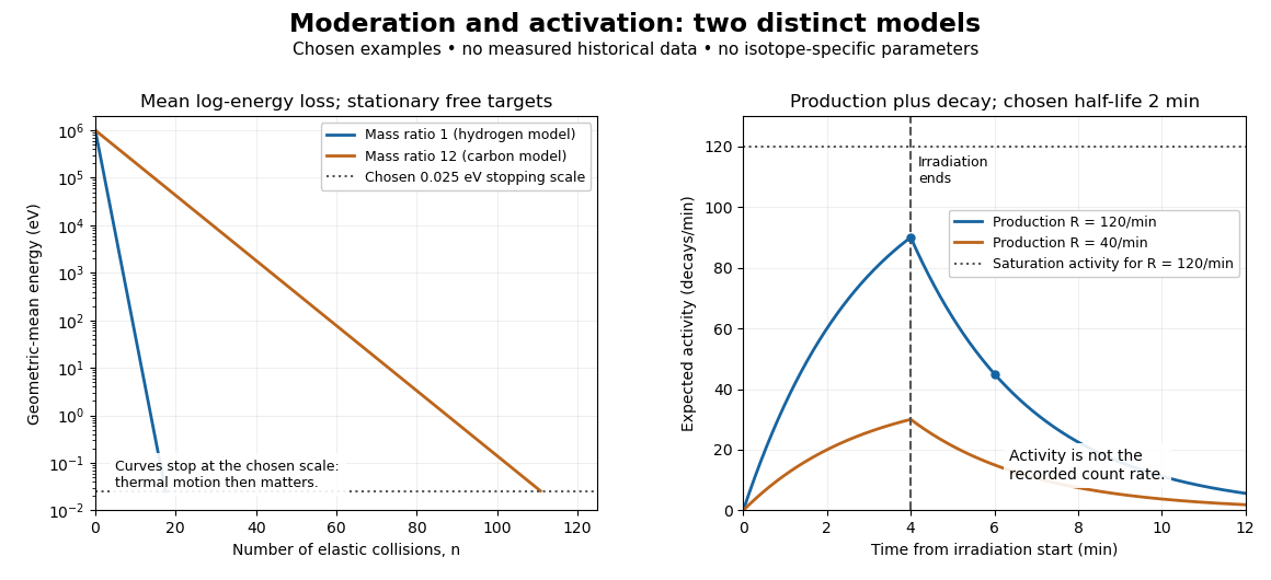
Let $\overline{N}$ be the expected value of the number of radioactive product atomic nuclei, initially zero, produced at constant rate $R$. Let their nuclear decay constant be $\lambda >0$. Assume one product species, negligible target depletion and negligible capture by the product. During irradiation, production adds $Rdt$ while radioactive decay removes $\lambda \overline{N}dt$ in expectation. Multiplying the resulting ordinary differential equation by $e^{\lambda t}$ givesThe expected radioactive activity $\overline{A}=\lambda \overline{N}$ tends to the production rate $R$. This saturation is a balance of continuing production and radioactive decay, not exhaustion of target atomic nuclei.

If irradiation ends at $t_i$, let $s$ denote elapsed time afterward. Setting the production term to zero givesFor detection efficiency $\epsilon$, constant background count rate $b$, delay $d$ and counting-window duration $\Delta$, integrating the expected count rate givesThis assumes at most one recorded pulse per product transformation and negligible counter losses. Detector response, branching fractions and background must be calibrated independently. Subtracting an estimated background does not remove its counting uncertainty. Several products give a sum of these terms with distinct nuclear decay constants; a single exponential decay fit can then mislead.

For a wholly stipulated example, choose $R=120{\min }^{-1}$, half-life $2\min$ and $t_i=4\min$. Then $\lambda =\log 2/(2\min )$, $\overline{A}(t_i)=90{\min }^{-1}$ and $\overline{N}(t_i)\simeq 259.69$. Choose $\epsilon =0.25$, $b=2{\min }^{-1}$ and $d=\Delta =2\min$. The result isThe background contributes four expected counts. Multiplying the initial net count rate in that window by its duration would give $22.5$ net counts, overestimating the integrated $16.23$ because the product decays appreciably during counting. All these values and the following curves are original examples, not measured historical data or parameters assigned to a particular silver isotope.

In the constant-rate mathematical model, an undecayed atomic nucleus has conditional probabilityof decaying during the next positive interval $\Delta t$. The nuclear decay constant has units of inverse time. Its value describes a rate; it does not specify a scheduled death time for one atomic nucleus. The conditional probability is independent of the age $t$, the memorylessness of the exponential distribution.

The number of radioactive atoms is determined by the supplied isotope mass, rather than by the total body mass:The radioactive activity is $\mathcal{A}=\lambda N$, with nuclear decay constant $\lambda =\ln 2/T_{1/2}$. Using $1\mathrm{yr}=365.25\times 86400\mathrm{s}$,ThereforeA becquerel is one decay per second; this is total activity over all decay branches. Multiplying by the argon-producing branching fraction would give that branch's activity, not the total asked for. Activity alone is also distinct from an absorbed radiation dose.

Let $K(t)$ be the surviving potassium-40 population and $A_r(t)$ the accumulated radiogenic argon-40. The total nuclear decay constant $\lambda$ sets $K(t)=K_0{e}^{-\lambda t}$. Only fraction $b=0.11$ of lost potassium atoms produces argon, so under the stated retention and zero-initial-argon assumptions,Dividing by the present potassium abundance eliminates the unknown initial population:With $A_r/K=0.3$,Thus the inferred potassium-argon dating age is about $2.5$ billion years, consistent with the proposed $2.5\times 10^9$-year age to the accuracy of the supplied inputs. Omitting the branching fraction would seriously underestimate the age. At exactly $2.5$ billion years, the model predicts $A_r/K\simeq 0.307$, consistent with the rounded measured $0.3$.

This dates closure of the mineral to argon loss and potassium exchange under the assumptions, not necessarily its original crystallization or the first formation of the Earth's crust. The depth alone is not an age measurement. No uncertainty or argon-retention history is supplied, so the agreement is a consistency check rather than proof of a particular geological event.

With no initial radiogenic argon-40 and complete daughter retention, the surviving potassium-40 population is $N_K=N_{K,0}{e}^{-\lambda t}$ and the accumulated daughter population is $N_{\mathrm{Ar}}=b(N_{K,0}-N_K)$. Here $\lambda$ is the total nuclear decay constant and $b$ is the argon-producing branching fraction. Their ratio gives the displayed age. The result measures closure of the mineral's isotope system under those assumptions.

Radioactive decay is the spontaneous transformation of an unstable atomic nucleus or nuclear state. Its timing can be unpredictable for an individual atomic nucleus while a large population has a reproducible average behavior. A constant nuclear decay constant $\lambda >0$ gives the familiar exponential decay law. The half-life describes how quickly the parent population falls, while radioactive activity describes its rate of transformations.^[ref]

This connection between randomness and a regular population law makes radioactive decay useful for measuring elapsed time and for understanding sources of radiogenic heating. It also distinguishes two questions in an experiment: what the source emits, and what an instrument records. Becquerel's uranium-radiation experiment used a photographic plate; the Curie ionization-current measurement measured an electrical consequence of radiation. Their readouts reveal different aspects of the same investigation.

A radiocarbon age estimates elapsed time from a measured carbon-14 ratio $R$, an assumed initial ratio $R_0$ and a specified nuclear decay constant $\lambda$. The displayed exponential decay inversion gives the age on that model's timescale. A conventional radiocarbon age uses a prescribed reference and decay convention; it is not generally a calendar age. Radiocarbon calibration accounts for changes in the atmospheric isotope ratio and maps the measurement to a calendar-age estimate.

An idealized radiochemical neutrino counting model separates production, survival, recovery and readout. Suppose a freshly cleared target produces atoms at a constant rate $R$ during exposure $T$. Each atom has nuclear decay constant $\lambda =\log 2/h$, where $h$ is its half-life. The expected surviving population obeysThe proof is to multiply the differential equation by $e^{\lambda t}$ and apply integration. The expression also follows by summing the exponential decay survival probabilities of atoms produced at every earlier time. Production does not imply eventual recovery: atoms can decay during exposure.

Let $\eta$ be the fraction recovered instantaneously at extraction, $d$ the subsequent delay before counting, $ϵ$ the probability of recording a decay, and $W$ the counting duration. The expected signal pulses areWith constant background rate $b$, the expected total is $\mu ={\mu }_s+bW$. During counting, the expected instantaneous pulse rate is $s(t)+b$, with $s(t)=ϵ\eta \lambda N(T)e^{-\lambda (d+t)}$. Equal time windows therefore lose signal by the factor $e^{-\lambda \Delta t}$ while a constant background stays unchanged. Fitting the time dependence helps distinguish radioactive decay from that background; it does not recover individual capture times.

For an original worked example choose $Rh=20$, $T=W=h$, $d=0$, $\eta =0.8$, $ϵ=0.5$ and $bh=0.2$. These are illustrative assumptions. Then $N(T)=10/\log 2$, andDoubling the exposure does not double the surviving inventory: $N(2h)/N(h)=3/2$. A delay of one half-life halves the signal. At $\lambda T\ll 1$, $N(T)\simeq RT$; at long exposure it saturates at $R/\lambda$. These limits explain why a large target and repeated extraction can matter more than simply waiting longer. The model neglects time-dependent production, finite extraction duration, residual atoms between runs and time-dependent backgrounds.

Radiometric dating estimates elapsed time from changes in radionuclide populations, using a known nuclear decay constant and assumptions about the initial composition and subsequent closure to matter exchange.

A radionuclide is a species of atomic nucleus with an unstable nuclear state that undergoes radioactive decay. A sample's expected surviving population decreases with its nuclear decay constant. Carbon-14 is the radioisotope used in radiocarbon dating.