Past exam of the advanced quantum physics course of the University of Cambridge / 2017

Solution

The operators associated with the two angular momenta commute with one another, and each squared angular momentum operator commutes with every component of that same angular momentum. Two useful identities are

J_{z} = J_{1 z} + J_{2 z}, J_{1} \cdot J_{2} = \frac{1}{2} (J^{2} - J_{1}^{2} - J_{2}^{2}) .

Consequently the two maximal commuting subsets of the displayed collection are

{J_{1}^{2}, J_{2}^{2}, J_{1 z}, J_{2 z}, J_{z}}, {J_{1}^{2}, J_{2}^{2}, J^{2}, J_{z}, J_{1} \cdot J_{2}} .

The first set gives the uncoupled eigenbasis

∣ j_{1} m_{1} ⟩ \otimes ∣ j_{2} m_{2} ⟩

. Its

J_{z}

eigenvalue is already fixed by

m = m_{1} + m_{2}

. The second gives the coupled eigenbasis

∣ j_{1} j_{2}; jm ⟩

for the addition of angular momentum. Its scalar-product eigenvalue is already fixed by

j, j_{1}, j_{2}

. Thus an independent complete set of commuting observables uses four operators in either case; literal maximality within the question's list includes the dependent fifth operator.

For generic nonzero angular momenta, no further listed operator can be added. In particular,

[J_{1 z}, J_{1} \cdot J_{2}] = i ℏ (J_{1 y} J_{2 x} - J_{1 x} J_{2 y})

is generally nonzero, and

[J_{1 z}, J^{2}] = 2 [J_{1 z}, J_{1} \cdot J_{2}]

. The same obstruction applies to

J_{2 z}

. Their sum

J_{z}

commutes because the two commutators cancel.

c

Solution

Write

C = e^{2} / (4 π ϵ_{0})

. The shell theorem makes the potential energy of the Electron constant inside the charged spherical shell. Relative to the point-proton Coulomb potential, the perturbation is

Δ V (r) = ⎩ ⎨ ⎧ C (\frac{1}{r} - \frac{1}{b}), 0, 0 < r < b, r \geq b .

It is positive: the finite charge distribution weakens the attraction close to the origin.

The first-order energy correction is the expectation value of this perturbation in the unperturbed hydrogen atom ground state. Integrating its probability density over spherical volume gives

Δ E = \frac{4 C}{a _{0}^{3}} \int_{0}^{b} e^{- 2 r / a_{0}} (r - \frac{r ^{2}}{b}) d r .

For a proton radius much smaller than the Bohr radius, expand the exponential uniformly over this short interval. The leading integral is

\int_{0}^{b} (r - \frac{r ^{2}}{b}) d r = \frac{b ^{2}}{6}, Δ E = \frac{2 C b ^{2}}{3 a _{0}^{3}} + O (\frac{C b ^{3}}{a _{0}^{4}}) .

Since

E_{1 s} = - C / (2 a_{0})

, the signed fractional change is

\frac{Δ E}{E _{1 s}} = - \frac{4}{3} (\frac{b}{a _{0}})^{2} + O (\frac{b ^{3}}{a _{0}^{3}}) .

Equivalently,

Δ E /∣ E_{1 s} ∣ = + 4 b^{2} / (3 a_{0}^{2})

to leading order: the energy increases and the binding-energy magnitude decreases. This is the finite proton-shell correction to hydrogen ground energy.

If no small-radius expansion is made, the same time-independent perturbation theory integral gives, with

β = b / a_{0}

\frac{Δ E}{∣ E _{1 s} ∣} = 2 [1 - \frac{1}{β} + (1 + \frac{1}{β}) e^{- 2 β}] .

Its expansion starts with

4 β^{2} /3

, in agreement with the leading result. The integral is exact for the first-order calculation; it is not an exact solution of the perturbed Schrödinger equation.

2

a

Solution

A spherical tensor operator of rank

k

transforms under rotation like an angular momentum

k

. The Wigner-Eckart theorem writes its matrix elements as

⟨ λ^{'} j^{'} m^{'} ∣ T_{q}^{(k)} ∣ λjm ⟩ = \frac{⟨ jm ; k q ∣ j ^{'} m ^{'} ⟩}{2 j ^{'} + 1} ⟨ λ^{'} j^{'} ∥ T^{(k)} ∥ λj ⟩ .

The reduced matrix element contains the radial and other dynamical information; the Clebsch-Gordan coefficients determine the dependence on the projections. Ratios within a fixed pair of multiplets therefore follow without a radial integral. The angular selection rules include

m^{'} = m + q

and

∣ j - k ∣ \leq j^{'} \leq j + k

For the position vector, choose the rank-one components

T_{0} = z, T_{\pm 1} = \mp \frac{x \pm i y}{2}, x = \frac{T _{- 1} - T _{+ 1}}{2} .

Let

R = ⟨ λ^{'}, 3/2∥ T^{(1)} ∥ λ, 1/2 ⟩

. The stretched Clebsch-Gordan coefficients and one lowering step give

⟨ \frac{1}{2}, \frac{1}{2}; 1, 1 \frac{3}{2}, \frac{3}{2} ⟩ = 1, ⟨ \frac{1}{2}, \frac{1}{2}; 1, 0 \frac{3}{2}, \frac{1}{2} ⟩ = \frac{2}{3} .

For example, apply the total angular momentum ladder operator to the stretched state. The result has components with coefficients

1/ 3

and

2/3

, corresponding to lowering the initial angular momentum and the vector component, respectively.

Only the

q = + 1

component of

x

contributes to

M_{1}

. The

q = 0

operator

z

cannot connect the projections in

M_{2}

, so that matrix element vanishes. With the convention above,

M_{1} = - \frac{R}{2 2}, M_{2} = 0, M_{3} = \frac{R}{6} .

Thus the requested relative magnitudes and their squared values are

∣ M_{1} ∣ : ∣ M_{2} ∣ : ∣ M_{3} ∣ = 3 : 0 : 2, ∣ M_{1} ∣^{2} : ∣ M_{2} ∣^{2} : ∣ M_{3} ∣^{2} = 3 : 0 : 4 .

These ratios presume a common nonzero reduced matrix element. The position operator has odd parity, so an electric dipole transition requires opposite-parity multiplets; for one Electron the electric-dipole selection rule also gives

Δ ℓ = \pm 1

. The displayed

j, m

labels alone do not establish that condition. If the common reduced matrix element vanishes, all three matrix elements vanish and no nonzero ratio can be inferred.

b

Solution

A uniform magnetic field quantizes the transverse cyclotron motion of an Electron. With Electron charge

- e

and the Landau gauge for a uniform magnetic field

A = (0, B x, 0)

, minimal coupling gives

H_{⊥} = \frac{p _{x}^{2}}{2 m} + \frac{( p _{y} + e B x ) ^{2}}{2 m} .

For an eigenstate of

p_{y}

with eigenvalue

ℏ k_{y}

, this is a quantum harmonic oscillator centered at

x_{c} = - ℏ k_{y} / (e B)

, with cyclotron frequency

ω_{c} = e B / m

. Its Landau levels are

E_{n} = ℏ ω_{c} (n + \frac{1}{2}), n = 0, 1, 2, \dots .

The oscillator width is set by the magnetic length

ℓ_{B} = ℏ/ (e B)

. In three dimensions, the free motion parallel to the magnetic field adds

ℏ^{2} k_{z}^{2} / (2 m)

. The Electron spin adds a Zeeman splitting

\pm g_{s} μ_{B} B /2

. In a crystal the appropriate band effective mass and effective spin factor replace the free-electron values.

Changing

k_{y}

moves the orbit center without changing the energy. In a rectangle

L_{x} L_{y}

, adjacent allowed centers differ by

2 π ℓ_{B}^{2} / L_{y}

. Requiring the center to lie in the sample gives the degeneracy of a Landau level, per spin,

N_{ϕ} = \frac{L _{x} L _{y}}{2 π ℓ _{B}^{2}} = \frac{e B L _{x} L _{y}}{h}, \frac{N _{ϕ}}{L _{x} L _{y}} = \frac{e B}{h} .

This large state degeneracy, together with the increasing level spacing, rearranges the occupied states as the magnetic field changes. To resolve the Landau levels, thermal broadening

k_{B} T

and disorder broadening should both be small compared with

ℏ ω_{c}

Figure 1.
Landau levels rise with magnetic field and pass through a fixed reference Fermi energy
. **Details**.

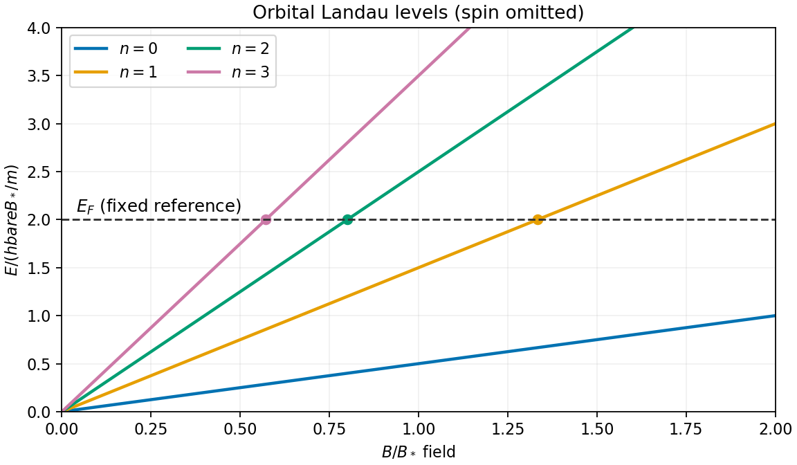
The de Haas-van Alphen effect is an oscillation of magnetization as successive Landau levels pass the Fermi energy. The Shubnikov-de Haas effect is the corresponding oscillation in longitudinal magnetoresistance. For a simple orbit, successive crossings occur periodically in

1/ B

; the general relation to the extremal orbit area is Onsager quantization. These measurements reveal the geometry and effective masses of a Fermi surface.

In a two-dimensional Electron system, filling an integer number

ν

of resolved levels leads to the integer quantum Hall effect, with

∣ σ_{x y} ∣ = ν \frac{e ^{2}}{h}, ∣ ρ_{x y} ∣ = \frac{h}{ν e ^{2}},

and very small longitudinal resistivity on a plateau. Disorder localization helps produce finite plateau widths. Cyclotron resonance provides another direct signature: radiation is absorbed at the adjacent-level spacing

ℏ ω_{c}

c

Solution

A coherent state is a normalized eigenstate of the annihilation operator,

a ∣ α ⟩ = α ∣ α ⟩

. Expanding in the Fock state eigenbasis gives a recurrence

c_{n + 1} = α c_{n} / n + 1

, and wavefunction normalization fixes

∣ α ⟩ = e^{- ∣ α ∣^{2} /2} \sum_{n = 0}^{\infty} \frac{α ^{n}}{n !} ∣ n ⟩ = D (α) ∣0 ⟩, D (α) = e^{α a^{†} - α^{*} a} .

The displacement operator therefore shifts the oscillator ground state in phase space. Distinct coherent states are not orthogonal:

⟨ α ∣ β ⟩ = exp [- \frac{∣ α ∣ ^{2} + ∣ β ∣ ^{2}}{2} + α^{*} β] .

The occupation probabilities form a Poisson distribution,

P_{n} = e^{- N} \frac{N ^{n}}{n !}, N = ∣ α ∣^{2}, ⟨ n ⟩ = N, (Δ n)^{2} = N .

For the quantum harmonic oscillator, the expectation values of position and momentum are

⟨ x ⟩ = \frac{2ℏ}{mω} Re α, ⟨ p ⟩ = 2 m ℏ ω Im α .

The fluctuations equal those of the ground state,

(Δ x)^{2} = \frac{ℏ}{2 mω}, (Δ p)^{2} = \frac{m ℏ ω}{2}, Δ x Δ p = \frac{ℏ}{2} .

Thus the position wavefunction is a displaced Gaussian wave packet that saturates the Heisenberg uncertainty principle.

Time evolution under

H = ℏ ω (a^{†} a + 1/2)

preserves this form:

e^{- i H t /ℏ} ∣ α ⟩ = e^{- iω t /2} ∣ α e^{- iω t} ⟩ .

(6)

The center follows the classical oscillator trajectory while the packet width stays constant. Its mean energy is

ℏ ω (N + 1/2)

; it is generally a superposition of energy eigenstates, rather than a state of definite energy. For

N ≫ 1

, the relative occupation fluctuation is

1/ N

, explaining the classical appearance of a highly excited coherent state.

3

Solution

The Zeeman effect comes from

- μ \cdot B

. For an Electron, the orbital and spin magnetic moments are approximately

- μ_{B} L /ℏ

and

- 2 μ_{B} S /ℏ

, respectively. This explains both the sign and the relative factor two in the term linear in

B

. The second term is the spin-orbit interaction: the Electron's motion through the atomic electric field produces a magnetic interaction in its rest frame. The relativistic correction, including Thomas precession, and the radial expectation value are incorporated into

K

. This effective Hamiltonian retains the linear Zeeman splitting and spin-orbit coupling, while omitting diamagnetic and hyperfine structure corrections.

Define the angular momentum ladder operators by

L_{\pm} = L_{x} \pm i L_{y}

and similarly for

S_{\pm}

. Direct expansion gives

\frac{1}{2} (L_{+} S_{-} + L_{-} S_{+}) = L_{x} S_{x} + L_{y} S_{y},

so adding

L_{z} S_{z}

gives the required scalar product. The off-diagonal terms change

m_{ℓ}

and

m_{s}

in opposite directions. Consequently

J_{z} = L_{z} + S_{z}

commutes with

H

, and

m_{j}

remains a good quantum number at every magnetic field.

In the given product eigenbasis, the diagonal matrix elements are

⟨ m_{ℓ}, m_{s} ∣ H ∣ m_{ℓ}, m_{s} ⟩ = μ_{B} B (m_{ℓ} + 2 m_{s}) + 2 K m_{ℓ} m_{s} .

For

ℓ = 1

and

s = 1/2

, the only off-diagonal couplings are between

(1, - 1/2)

and

(0, 1/2)

, and between

(0, - 1/2)

and

(- 1, 1/2)

. Each relevant orbital ladder factor is

ℏ 2

and each spin ladder factor is

ℏ

. Multiplying by

K / ℏ^{2}

gives

2 K

. Therefore

a = μ_{B} B, b = K, c = 2 K .

All other off-diagonal entries vanish either by the ladder endpoints or by conservation of

m_{j}

. This derives every entry of the displayed matrix.

The stretched states have no mixing and yield

E_{m_{j} = 3/2} = K + 2 a, E_{m_{j} = - 3/2} = K - 2 a .

The

m_{j} = 1/2

block is

(- K 2 K 2 K a)

, while the

m_{j} = - 1/2

block is

(- a 2 K 2 K - K)

. Taking the trace and determinant of each

2 \times 2

block gives the remaining four energy eigenvalues:

E_{+}^{(\pm)} = \frac{a - K}{2} \pm \frac{1}{2} (a + K)^{2} + 8 K^{2},

E_{-}^{(\pm)} = \frac{- a - K}{2} \pm \frac{1}{2} (a - K)^{2} + 8 K^{2} .

(6)

The subscripts indicate

m_{j} = \pm 1/2

and the superscripts indicate the upper or lower root. These formulas are the Zeeman spectrum for orbital angular momentum one and remain valid for either sign of

K

For the usual ordering

K > 0

, including sodium, the zero-field states follow from

L \cdot S = \frac{1}{2} (J^{2} - L^{2} - S^{2}), E_{j} = K [j (j + 1) - ℓ (ℓ + 1) - s (s + 1)] .

(7)

The

j = 3/2

quartet lies at

K

and the

j = 1/2

doublet at

- 2 K

, separated by

3 K

. In a weak magnetic field, the Landé g-factors give

E_{3/2, m_{j}} = K + \frac{4}{3} a m_{j} + O (a^{2} / K), E_{1/2, m_{j}} = - 2 K + \frac{2}{3} a m_{j} + O (a^{2} / K) .

(8)

These label the curves near

B = 0

. In a strong magnetic field, the Paschen-Back effect makes

(m_{ℓ}, m_{s})

the appropriate approximate labels:

E_{m_{ℓ}, m_{s}} = a (m_{ℓ} + 2 m_{s}) + 2 K m_{ℓ} m_{s} + O (K^{2} / a)

(9)

for the mixed states, with the stretched-state formulas already exact. The branch connections for

B > 0

are

zero-field label (j, m_{j}) (3/2, 3/2) (3/2, 1/2) (1/2, 1/2) (3/2, - 1/2) (1/2, - 1/2) (3/2, - 3/2) strong-field label (m_{ℓ}, m_{s}) (1, 1/2) (0, 1/2) (1, - 1/2) (- 1, 1/2) (0, - 1/2) (- 1, - 1/2)

(10)

Within a fixed

m_{j}

, the nonzero coupling prevents a crossing; this is an avoided crossing. Curves with different

m_{j}

may cross because the Hamiltonian does not couple them.

Figure 1.
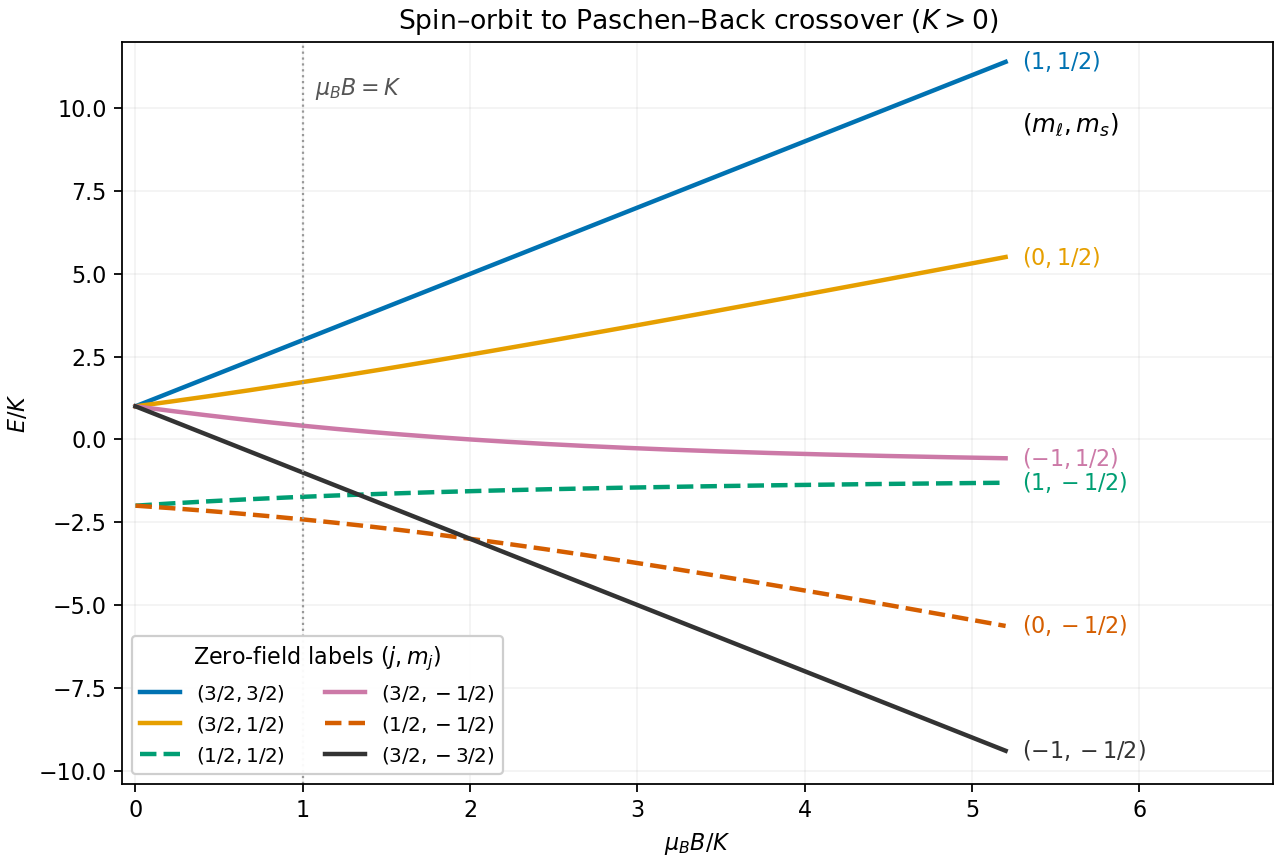
Exact spin-orbit and Zeeman energies for orbital angular momentum one and positive spin-orbit constant
. **Details**.

For the sodium estimate, the zero-field frequency separation fixes

3 K = h δ f, K = 1.14 \times 1 0^{- 22} J .

(11)

The lower

3 s

doublet has shifts

\pm a

. The Sodium D-line Zeeman pattern gives photon-frequency shifts

a / h

times

{\pm 2/3, \pm 4/3}

for D

_{1}

and

{\pm 1/3, \pm 1, \pm 5/3}

for D

_{2}

. Thus the highest-frequency D

_{1}

component and lowest-frequency D

_{2}

component approach each other by

3 a / h

. Extrapolating the weak-field Zeeman splitting gives

B_{cross} \sim \frac{h δ f}{3 μ _{B}} = 12.3 T,

(12)

so the crossover occurs at a field of order

10 T

, where

a \sim K

and the weak-field approximation is becoming marginal.

The exact eigenvalues refine the estimate within this Hamiltonian. The relevant photon energies, with a common zero-field reference omitted, are

E_{+}^{(-)} + a

and

E_{-}^{(+)} - a

. The corresponding electric dipole transitions have

Δ m_{j} = + 1

and

- 1

, respectively. Equating them gives

6 a = (a + K)^{2} + 8 K^{2} + (a - K)^{2} + 8 K^{2} .

(13)

Its positive solution is

a / K = 10 /3

, hence

B_{cross} = \frac{10 h δ f}{9 μ _{B}} ≃ 13.0 T

(14)

in the retained model. The crossing is between optical transition frequencies; the participating upper states themselves need not be degenerate.

4

Solution

For elastic scattering by the Yukawa potential, take

κ > 0

and use the first Born approximation in the plane-wave normalization

f_{B} (q) = - \frac{m}{2 π ℏ ^{2}} \int e^{- i q \cdot r} V (r) d^{3} r .

Choose the polar axis along the momentum transfer

ℏ q

. The angular integral is

\int e^{- i q r c o s ϑ} d Ω = 2 π \int_{- 1}^{1} e^{- i q r u} d u = 4 π \frac{s i n ( q r )}{q r} .

The radial volume element cancels the remaining powers of

r

, leaving

f_{B} (q) = - \frac{2 m A}{ℏ ^{2} q} \int_{0}^{\infty} e^{- κ r} sin (q r) d r = - \frac{2 m A}{ℏ ^{2} ( q ^{2} + κ ^{2} )} .

For real

A

, the differential scattering cross-section is therefore

\frac{d σ}{d Ω} = ∣ f_{B} (q) ∣^{2} = [\frac{2 m A}{ℏ ^{2} ( q ^{2} + κ ^{2} )}]^{2} .

This also has a finite forward limit when

κ > 0

. The Born amplitude for a Yukawa potential provides a screened route to the Coulomb potential by taking

κ \to 0^{+}

at fixed

q > 0

For an alpha particle of charge

2 e

scattering from a heavy nucleus of charge

Z e

, set

A = 2 Z e^{2} / (4 π ϵ_{0})

. Neglect recoil, so that the reduced mass is approximately the projectile mass,

E = ℏ^{2} k^{2} / (2 m)

, and elastic geometry gives

q^{2} = ∣ k_{out} - k_{in} ∣^{2} = 4 k^{2} sin^{2} \frac{θ}{2} .