Source: released examination bundle,
Part A 2007 11-1.pdf, pages 259–264. The printed title is Algebra, Analysis and Differential Equations I. The paper is cross-listed for mathematics and mathematics and statistics and contains no printed mark allocations.The annihilator of a vector subspace is the vector subspace of the dual space consisting of the linear functionals that vanish on :It is a vector subspace because every linear combination of functionals vanishing on still vanishes there.
For the basis , define the dual basis byUniqueness of the coordinates makes each well-defined and linear. If , evaluation at gives , so these linear functionals are linearly independent. For any , evaluation on each basis vector givesBoth sides agree on a basis, hence on every linear combination. Thus they also span the dual space and are a basis of it.
Let denote the coordinate linear functional dual to the th vector of the standard basis. Writing a vector in the supplied basis givesSuccessive differences recover the coefficients. Hence the dual basis isThese formulas directly give and exemplify the dual basis of cumulative coordinate sums.
The span is the coordinate plane . Consequently its annihilator of a vector subspace is . The dual map is composition with , soIt follows thatEquivalently, sends to .
The Gram-Schmidt process subtracts projections onto directions already constructed and then normalizes. Define recursivelywhere the empty sum for is zero. Assuming the preceding are orthonormal, taking the inner product of with , , gives zero. Moreover : otherwise would belong to the span of , contrary to linear independence. Normalization is therefore legitimate and produces an orthonormal basis. At each stage the first constructed vectors have the same span as the first original vectors.
A real inner product must be symmetric. Here and , forcing . For this value,This is strictly positive for every nonzero vector. Bilinearity is already given, so symmetry and positive definiteness prove
Use the inner product with . The required first vector already has squared norm . Apply the Gram-Schmidt process to followed by . Since , its orthogonal remainder is . Its squared norm is . Therefore an orthonormal basis containing the specified vector isThe second vector may also be replaced by its negative.
The Chinese remainder theorem for two comaximal two-sided ideals of a ring states that the natural ring homomorphism inducesIndeed, the map has kernel of a ring homomorphism . Choose , with . Given target representatives , the element is congruent to modulo and to modulo , proving surjectivity. The first isomorphism theorem for rings gives the result. For a commutative ring, : if , then , while the reverse inclusion follows from the ideal properties.
Take , and . Since are coprime integers, Bézout's identity gives , so . Their intersection is : it consists of integers divisible by both and , and coprimality makes this equivalent to divisibility by . Thus the Chinese remainder theorem givesas a ring isomorphism. This includes or , where the corresponding factor is the zero ring.
Let count everyone present, including the host. The grouping, seating and departure conditions give the modular congruencesThe first two imply , and oddness forces even. By the Chinese remainder theorem, the complete solution isBecause not every invitee attended, at most guests came, so . For , the only positive possibility is 39 people. It is feasible: seven groups of five and one of four; three tables of ten and one of nine; nineteen departing pairs and the host.
For , both 39 and 129 people are possible. The latter uses twenty-five groups of five and one of four, three tables of ten and eleven of nine, and sixty-four departing pairs. Thus the larger invitation count destroys uniqueness; it does not force a different attendance.
In the subspace topology on , a subset is open in precisely when for some open set . A subset is closed in precisely when is open in , equivalently for some closed set .
A compact space is one for which every open cover has a finite subcover. Here the cover may use relatively open subsets of , or equivalently ambient open subsets covering it. The Heine-Borel theorem states thatClosedness and boundedness here refer to the ambient complex plane, not merely closedness in itself.
A connected space cannot be expressed as with disjoint nonempty relatively open sets. Equivalently, the only subsets simultaneously relatively open and closed are and . A decomposition into such is a separation of the topological space.
A path-connected space has, for every pair , a continuous path with and . Every path-connected space is a connected space, because a separation of the target would pull a joining path apart and contradict connectedness of an interval.
The integers are unbounded in the complex plane, so the Heine-Borel theorem shows they are not compact. They are also not connected: and are disjoint nonempty relatively open sets covering . Each integer is isolated, so the induced subspace topology is discrete.
The disc is a closed set and is bounded in the complex plane, so it is compact by the Heine-Borel theorem. It is convex: the triangle inequality gives for all when both endpoints lie in it. Straight segments therefore supply paths, so it is path-connected and hence connected.
The union is bounded but is not a closed set: the points , , belong to the open disc and tend to , which lies in neither disc. Thus it is not compact by the Heine-Borel theorem.
Nevertheless it is connected, indeed path-connected. Every point of the open disc joins by a straight segment. The segment from to stays in the union, since its points before the endpoint belong to the open disc and the endpoint belongs to the closed disc. Every point of that closed disc joins inside it by convexity. Concatenating these paths joins any two points of the union. The fact that the two discs are disjoint does not imply disconnection: their contact point belongs to one of them. This illustrates connectedness at a one-sided contact point.
An isolated singularity at means that the function is holomorphic on some punctured disc , while it is undefined or fails to be holomorphic at . The punctured neighbourhood contains no other singularities; this isolation is needed before applying the usual removable/pole/essential classification.
A removable singularity at is an isolated singularity for which one can assign a value at to obtain a holomorphic function on the whole disc. Equivalently its Laurent series has no negative powers. A finite limit supplies the extension value .
A pole of order at meansEquivalently the lowest nonzero power in its Laurent series is . In particular, tends to a finite nonzero limit.
The possible singular points are . Near , put ; thenThe numerator vanishes at , so the apparent pole cancels and is removable. Its extension value is , obtained from .
At , the first term has a simple pole with nonzero residueThe subtracted term is holomorphic there, so is a simple pole. At ,so is a double pole. There are no other finite singularities.
Away from zero, singularities occur exactly when , namelyFor , differentiation at gives . Thus every is a simple pole, with residue .
As , these poles accumulate at zero. Therefore zero is a non-isolated singularity. Every punctured disc around it contains poles, so the function is not holomorphic on any punctured disc there. In particular zero cannot be classified as an isolated essential singularity; the isolated-singularity classification does not apply. The displayed poles and their accumulation point zero exhaust the finite singularities.
The contour integral along a piecewise smooth path is defined by parametrization:with a sum over the smooth pieces. The residue theorem states that for a positively oriented simple closed contour and a function holomorphic on and inside it apart from finitely many isolated singularities inside,More generally a closed contour uses the winding number of each singularity as its weight.
Set , so and . The required real integral becomesThe denominator factors as . Only the simple poles lie inside the unit circle. At either one,The residue theorem now gives
With , direct differentiation givesThe homogeneous ordinary differential equation therefore has general solution . Chooseso and . Their Wronskian in the convention is . There is no nonzero homogeneous solution satisfying both boundary conditions, since the first forces and the second forces .
For the operator as printed, whose leading coefficient is , the Green's function isIt satisfies the endpoint boundary conditions, is continuous across , and its first derivative has jump . Multiplying that jump by the leading coefficient produces the unit source required by a Green's function. This factor matters because the operator was not normalized to leading coefficient one; it is an instance of a Green function under dependent-variable rescaling.
Thus . For , split the integral at to obtainThereforeThe substitution above gives , so the forcing is indeed , and both endpoint values vanish.
Both components vanish atThe Jacobian matrix of the vector field isIts eigenvalues classify these equilibria by linearization of a dynamical system:All real parts are nonzero, so the linear classifications determine the local stability of the nonlinear autonomous system.
At the origin, the stable direction is the -axis and the unstable direction is the -axis. At the eigendirections are for and for . At ,has only one eigendirection, the -axis; its linearization of a dynamical system has solutions , , explaining the improper node. At , stable and unstable tangent vectors are respectively and .
For the phase portrait, the axes are invariant, and the remaining nullclines are and . Off these lines, the complete directional information isIn the positive quadrant, arrows point right above and left below it, and point up above and down below it. On the positive -axis, trajectories tend to . On the -axis, flows toward the origin and flows upward. These signs and the saddle directions give the following sketch; the plotted curves illustrate the phase portrait, with the marked saddle curves tangent to the calculated eigenvectors.
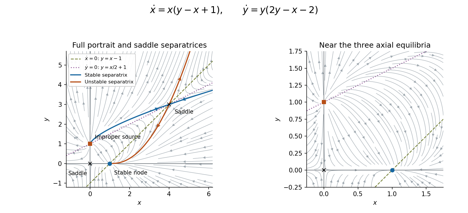
Phase portrait with the four equilibria, both non-axis nullclines, and stable and unstable separatrices of the saddle at (4,3). Arrows indicate increasing time.
Details. 
Introduce a characteristic parameter and label each point of the initial segment by . The method of characteristics givesIntegrating gives the parametric solutionThe projected characteristic curves satisfy , so each lies on a straight line through . Its branch from the data always has ; the common vertex is approached only as .
Eliminating using and yieldsIts derivatives give , and substitution of gives the prescribed value one.
The Jacobian determinant of is , and the inverse just displayed is unique. Hence the data determine the solution exactly onThis is the domain determined by a finite segment under a radial characteristic flow. Its interior is , ; the two boundary rays come from the endpoints of the initial segment. Every point there lies on exactly one characteristic from the data. Outside this sector, a characteristic either misses the initial segment or lies on the branch , which cannot reach it. Thus the formula may be extended beyond this sector, but such an extension is not uniquely specified by the given data.
Articles by others on the same topic
There are currently no matching articles.