Past exam of the differential equations and applications course of the University of Oxford / 2010 (B5, DMAB 2644, DMCN 2644, DMST 2644)

Original solutions to the paper released at the source request. The complete editable transcription is retained in the private examination archive.

The characteristic polynomial is $r^2+2r+2=(r+1{)}^2+1$, with distinct complex roots $r=-1\pm i$. Taking the real and imaginary parts of the corresponding exponential functions gives the real fundamental system of solutions $e^{-x}\cos x$ and $e^{-x}\sin x$. Consequently the general real solution isTheir Wronskian is $e^{-2x}\ne 0$, so they span the two-dimensional real solution space.

For each $0<\xi <2\pi$, the Green's function is a distribution in $x$ satisfyingEquivalently, $g$ is a classical homogeneous solution on each side of $\xi$, satisfies the same endpoint conditions, and obeys the Green function jump conditionsTo see equivalence, let $[g]$ and $[g_x]$ denote its jumps. The singular part of $L_{x}g$ is $[g]{\delta }^{\prime }(x-\xi )+([g_x]+2[g])\delta (x-\xi )$. Matching a unit Dirac delta distribution with no derivative first forces continuity, then the unit derivative jump. Conversely these conditions produce exactly that distribution. The solution for a regular forcing is $y(x)={\int }_0^{2\pi }g(x,\xi )f(\xi )d\xi$. The homogeneous endpoint problem has only the zero solution, which ensures uniqueness of this kernel.

Choose a left-end solution $u(x)=e^{-x}\sin x$ and a right-end solution $v(x)=e^{-x}(\sin x+\cos x)$. They satisfy $u(0)=0$ and $v^{\prime }(2\pi )=0$. Their Wronskian, with the order used here, isThe Green's function is $u(x_{<})v(x_{>})/W(\xi )$, where $x_{<}=\min (x,\xi )$ and $x_{>}=\max (x,\xi )$. Explicitly,The two expressions agree at the source. Their derivative difference is $[u(\xi )v^{\prime }(\xi )-u^{\prime }(\xi )v(\xi )]/W(\xi )=1$, checking both normalization and sign. The first-order derivative term means the kernel need not be symmetric under exchange of $x$ and $\xi$.

A distribution is a continuous linear functional on the space of test functions $\mathcal{D}(\mathbb{R})=C_c^{\infty }(\mathbb{R})$. A precise useful form of continuity is: for every compact set $K\subset \mathbb{R}$ there exist an integer $m\ge 0$ and a constant $C_K$ such thatEquivalently, if a sequence of test functions has supports in one fixed compact set and every derivative tends uniformly to zero, then its images under $T$ tend to zero. Keeping a common compact support is part of the test function topology; mere pointwise convergence is insufficient.

Linearity follows from linearity of differentiation and point evaluation. For a test function supported in a fixed compact set $K$, its value and derivative vanish at any point outside $K$. ThereforeThis proves the continuity estimate with $m=1$ and $C_K=2$ for every $K$. Thus the stated mapping is a distribution of order at most one, supported in $\{0,1\}$. In particular, a sequence tending to zero in the test function topology has both ${\varphi }_n^{\prime }(0)\to 0$ and ${\varphi }_n(1)\to 0$.

The distributional derivative is defined by moving the derivative onto a test function and changing the sign:Since $⟨{\delta }_a,\varphi ⟩=\varphi (a)$, one has $⟨{\delta }_0^{\prime },\varphi ⟩=-{\varphi }^{\prime }(0)$. HenceThe minus sign in front of ${\delta }_0^{\prime }$ is essential: it makes its action the positive derivative evaluation required here.

Set $t=\log x$, so $0<t<\pi$, and write $y(x)=x^{-2}w(t)$. Direct differentiation of this Cauchy-Euler equation givesThe eigenvalue equation is therefore $-w^{\prime \prime }=(\lambda -3)w$ with $w(0)=w(\pi )=0$. For $\lambda -3\le 0$, the linear/hyperbolic solutions cannot satisfy both endpoint conditions except trivially. For $\lambda -3>0$, the sine solution vanishes at both endpoints exactly when its frequency is a positive integer. ThusEach associated eigenspace is one-dimensional.

The displayed differential operator is not self-adjoint for the unweighted inner product. Let $A=x^2{\partial }_x^2+5x{\partial }_x+1$. Integration by parts on compactly supported smooth functions gives its formal adjointwhich differs from $A$. One can see an explicit failure of symmetry without boundary terms: take a nonzero real compactly supported smooth $f$ in the interval and $g=xf$. ThenBoth test functions obey the Dirichlet endpoint conditions. Changing the sign of $A$ for the eigenproblem does not repair this failure. A different, weighted inner product with weight $x^3$ does give the Sturm-Liouville form $x^{3}Ay=(x^5{y}^{\prime }{)}^{\prime }+x^{3}y$, explaining why a real discrete spectrum is nevertheless natural.

Use the cosine difference identity to separate the kernel:Thus $L$ has image $E=\mathrm{span}\{c,s\}$, where $c(x)=\cos 2x$, $s(x)=\sin 2x$. Their squared norms in $L^2(0,\pi )$ are $\pi /2$ and they are orthogonal. ConsequentlyEvery nonzero eigenvalue must belong to this two-dimensional image, so the complete list of eigenvalues of finite multiplicity isEach has multiplicity one. On $E^{\perp }$ the operator vanishes, giving the zero eigenvalue infinite multiplicity. For example $\boxed{y(x)=1}$ is a nonzero element of the kernel because both relevant integrals over the interval vanish.

The forcing is $\frac{1}{2}\sin 2x$, which lies in the image of $L$. Since the eigenvalue on $\sin 2x$ is $\pi /4$, a particular solution is $y_p=(2/\pi )\sin 2x$. The full family isThus solutions exist and are not unique: adding any element of the infinite-dimensional kernel leaves $Ly$ unchanged. For example every constant can be added.

Every image of $L$ is a linear combination $a\cos 2x+b\sin 2x$. The function $\cos x$ is not such a combination. Indeed these functions are continuous, so equality almost everywhere would imply equality everywhere; evaluation at the endpoints would require simultaneously $a=1$ and $a=-1$. Therefore the forcing is outside the image and there is no solution. Orthogonality to the kernel is the equivalent image test for this self-adjoint finite-rank operator.

Rewrite the equation as $(L-I)y=\cos x$. On $E=\mathrm{span}\{\cos 2x,\sin 2x\}$, the operator $L-I$ has eigenvalues $\pi /2-1$ and $\pi /4-1$, both nonzero. On $E^{\perp }$ it equals $-I$. The orthogonal decomposition $L^2(0,\pi )=E\oplus E^{\perp }$ therefore makes $L-I$ bijective with bounded inverse. In particular there is exactly one solution for this forcing. This is also the finite-rank Fredholm alternative: $1$ is not an eigenvalue of $L$, so adding the identity term removes the image obstruction present in $Ly=f$.

Normalize the Laguerre differential equation as $y^{\prime \prime }+P(x)y^{\prime }+Q(x)y=0$, where $P(x)=1/x-1$ and $Q(x)=n/x$. At $x=0$, the products $xP=1-x$ and $x^{2}Q=nx$ are analytic. Thus zero is a regular singular point, with indicial equationAt $x=1$ the coefficients $P,Q$ are analytic, so it is an ordinary point. No singular-point indicial equation is needed there.

For infinity put $z=1/x$ and $Y(z)=y(1/z)$. Then the equation becomesAt $z=0$, the coefficient $z(z^{-1}+z^{-2})=1+1/z$ is not analytic. Therefore infinity is an irregular singular point, including when $n=0$. A terminating polynomial solution does not change the classification of the differential equation.

Substitute $y={\sum }_{k\ge 0}{a}_k{x}^k$ and compare the coefficient of $x^k$. The two derivative terms give $(k+1{)}^2{a}_{k+1}$, while the remaining terms give $(n-k)a_k$. ThusIterating the recurrence givesIndeed the recurrence first vanishes at $k=n$ and then remains zero. Consequently the Laguerre polynomial iswith exact degree $n$ and leading coefficient $(-1{)}^n/n!$. This is the regular power-series branch normalized at zero; the second branch at the repeated indicial root is not an additional analytic solution with this normalization.

Assume first that $n\ge m$. Substituting Rodrigues' formula for $L_n$ givesHere integration by parts was performed $n$ times. Each boundary term vanishes: at infinity a polynomial times $e^{-x}$ tends to zero; at zero every derivative of $x^n{e}^{-x}$ of order less than $n$ vanishes. If $n>m$, the derivative $L_m^{(n)}$ is zero, proving orthogonality. The case $m>n$ follows by exchanging the two factors.

For $m=n$, the leading coefficient found above gives $L_n^{(n)}=(-1{)}^n$. ThereforeThe same conclusion includes $n=0$ directly. Thus the full Laguerre orthonormality relation is

Use the initial-curve parameter $s$ and a characteristic parameter $t$. Charpit's equations areAt $t=0$ prescribe $x=x_0(s)$, $y=y_0(s)$ and $u=u_0(s)$. The two initial derivatives $p_0,q_0$ must satisfyThe second equation is the chain rule along the initial curve. For the usual local Cauchy construction also require the non-characteristic condition $x_0^{\prime }{F}_q-y_0^{\prime }{F}_p\ne 0$. It ensures both local determination of an allowed branch of $p_0,q_0$ and local inversion of the projected characteristic coordinates.

Along a characteristic, the chain rule and the five equations giveSince $F=0$ initially, $\boxed{F\equiv 0}$ along each constructed curve. With the contact compatibility $du=pdx+qdy$ propagated by this system, an invertible characteristic chart reconstructs $p=u_x,q=u_y$ and hence a local classical solution.

Set $F=xp+q^2/4+u-1$. Parametrize the data by $x_0=s$, $y_0=0$, $u_0=1-s^2/3$. Tangential differentiation gives $p_0=-2s/3$; substitution into $F=0$ then gives $q_0^2=4s^2$. Thus the data allow two normal-derivative branches, indexed by $\epsilon =\pm 1$, with $q_0=2\epsilon s$. For $s>0$ each branch is non-characteristic; the endpoint $s=0$ is degenerate.

The Charpit's equations reduce to $\dot{x}=x$, $\dot{y}=q/2$, $\dot{p}=-2p$, $\dot{q}=-q$ and $\dot{u}=xp+q^2/2$. Integrating with these initial values givesDirect substitution checks $xp+q^2/4+u-1=0$, and $t=0$ recovers the initial data. The projection onto the $(x,y)$ plane has Jacobian determinantIt first vanishes at $t=\log 2$. These points form the characteristic caustic $y=\epsilon x/4$, $0<x\le 2$; a single classical solution cannot in general be continued through the fold by treating all projected characteristic curves as a graph.

For a precise description put $r=\epsilon y$. On the chart containing the initial curve and lying before the fold, $t<\log 2$, elimination givesThe plus square-root is forced by $s/x>1/2$, rather than a free second choice. The conditions $0<s\le 1$ give the complete unfolded chartInterior points of the domain have strict inequality at the boundary generated by $s=1$ as well. The other boundary is the characteristic caustic; the original endpoint $s=0$ contributes no open chart. On the portion obtained by following characteristics forward from the data, $0\le t<\log 2$, the region is more specificallyThe $s=1$ boundary is $y=\epsilon (1-1/x)$ and meets the characteristic caustic at $(2,\epsilon /2)$. Negative characteristic times give the continuation across the initial segment into the opposite half-plane. Each sign branch is a distinct local solution; the initial values alone do not select one of them.

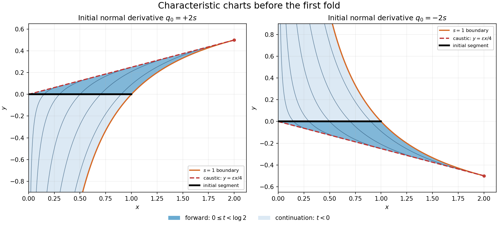
The solid shading follows $t\ge 0$; the lighter shading shows the same smooth chart at $t<0$. Reflected panels correspond to the two allowed signs of the initial normal derivative. Beyond the dashed characteristic caustic the characteristic parametrization no longer gives this smooth graph.

Write the system as $U_x+A(U)U_y=0$ with $U=(u,v{)}^T$ andIts two characteristic speeds are ${\lambda }_{\pm }=v\pm \sqrt{u}$, so it is strictly hyperbolic precisely when $u>0$. At $u=0$ they coincide and the matrix is not diagonalizable; for $u<0$ the speeds are nonreal.

For $u>0$ define $R_{\pm }=v\pm 2\sqrt{u}$ and $D_{\pm }={\partial }_x+(v\pm \sqrt{u}){\partial }_y$. Substitution from the two differential equations givesThereforeThese are the two Riemann invariants; their constancy applies within smooth regions, not across a shock.

For a smooth solution, the first equation is $u_x+(uv{)}_y=0$. Multiplying it by $v$ and adding $u$ times the second equation givesThus the appropriate shallow water equations conservation variables and flux areUse this conservative extension to define a weak solution across $y=F(x)$. A jump contributes $-F^{\prime }[W]\delta (y-F(x))$ to $W_x$ and $[H]\delta (y-F(x))$ to $H_y$. Cancellation of the singular parts gives the Rankine-Hugoniot conditionsEquivalently this follows by integrating each conservation law over a thin space-time control region crossing the discontinuity.

The conservative extension is essential here. Piecewise smoothness by itself does not imply any jump law. Moreover the smooth second equation can also be written $v_x+(u+v^2/2{)}_y=0$; imposing that different conservation law distributionally would give a different shock condition. Weak conservation laws depend on conserved variables. The requested jump law specifically selects mass $u$ and momentum $uv$, and this is the extension used below.

Test a single discontinuity connecting the two constant initial states. With state 1 below the discontinuity and state 2 above it, their jumps areThe first Rankine-Hugoniot condition gives $F^{\prime }=\sqrt{3}$, and the second independently gives $(-\sqrt{3})F^{\prime }=-3$, the same value. Since the initial jump is at the origin,Values on the shock itself do not affect the weak solution. No intermediate state or rarefaction is needed: the prescribed states already lie on the same compressive shock curve.

For admissibility, the upper-family characteristic speed is $\sqrt{3}/2+\sqrt{2}$ behind the shock and $1$ ahead of it. They satisfyBoth lower-family speeds, $-1$ and $\sqrt{3}/2-\sqrt{2}$, are less than the shock speed. These are the Lax shock admissibility conditions for a family-plus shock. This is the entropy-admissible solution for the mass/momentum conservative extension specified by the preceding jump law; imposing an additional velocity conservation law across the same jump would describe a different problem.

For $\eta =x/y^{\beta }$ the chain rule gives $u_y=-\beta \eta f^{\prime }/y$, $u_x=y^{-\beta }{f}^{\prime }$ and $(u{u}_x{)}_x=y^{-2\beta }[f{f}^{\prime \prime }+(f^{\prime }{)}^2]$. Multiplication of the equation by $y$ givesA nontrivial scale-invariant balance therefore selects $\boxed{\beta =1/2}$ and yieldsIts left side is the derivative of $f{f}^{\prime }+\eta f/2$. The boundary conditions give $f(0)=1$ and $f^{\prime }(0)=0$, so the integration constant is zero:On the positive branch before the first zero, divide by $f$ and integrate, obtaining $f=1-{\eta }^2/4$. Its first positive zero is ${\eta }_F=2$. HenceA direct check gives $u_y=x^2/(4y^2)$ and $(u{u}_x{)}_x+u/(2y)=x^2/(4y^2)$. The zero extension past this front is also a natural weak compact-support continuation: $u$ is continuous and the degenerate diffusive flux $u{u}_x$ tends to zero at the front. This is a source-driven porous-medium similarity front.

Assume a classical solution $u\in C^2(D)\cap C(\overline{D})$, as needed to interpret the boundary values. At an interior local minimum its Hessian is positive semidefinite, hence $\Delta u\ge 0$. But the equation gives $\Delta u=-e^{-x^2}<0$, a contradiction. Since $D$ is bounded and $u=0$ on its boundary, a nonpositive interior value would either furnish an interior negative minimum or itself be a zero minimum. Thus $\boxed{u>0\text{ in }D}$.

For the upper bound use the barrier $w(x,y)=(1-x^2-y^2)/4$, which satisfies $-\Delta w=1$. Set $z=w-u$. On the boundary $z=w\ge 0$, because the domain lies inside the unit disk, whileThe quadratic perturbation proof of the minimum principle gives $z\ge 0$. The strong minimum principle for elliptic operators makes this strict in the connected interior unless $z$ is constant. Constancy is impossible since $1-e^{-x^2}$ is not identically zero on any open domain. HenceThis last strong-principle step handles points with $x=0$, where the comparison forcing itself vanishes. Simple connectedness is not needed for the comparison argument.

With source point $\xi \in D$ and field point $X=(x,y)$, the Dirichlet Green function for the operator $-\Delta$ satisfiesClassically it is harmonic off $\xi$, with the two-dimensional normalization $G(X,\xi )=-(2\pi {)}^{-1}\log |X-\xi |+H(X,\xi )$, where $H$ is regular near the source. Equivalently $-{\lim }_{r\downarrow 0}{\int }_{|X-\xi |=r}{\partial }_{r}Gds=1$. This sign convention gives the representation $u(X)={\int }_{D}G(X,\xi )e^{-{\xi }_1^2}d\xi$.