The geometric path difference for a direction at zenith angle is . Equal cable lengths leave that difference unchanged; the inserted electronic delay cancels for the tracking center. The residual delay is thereforeThe complex visibility of the unresolved source has phase , giving in the chosen baseline ordering. Reversing the signal order complex-conjugates it without changing the measured visibility magnitude. Tracking the antennas geometrically does not itself provide this fringe stopping.
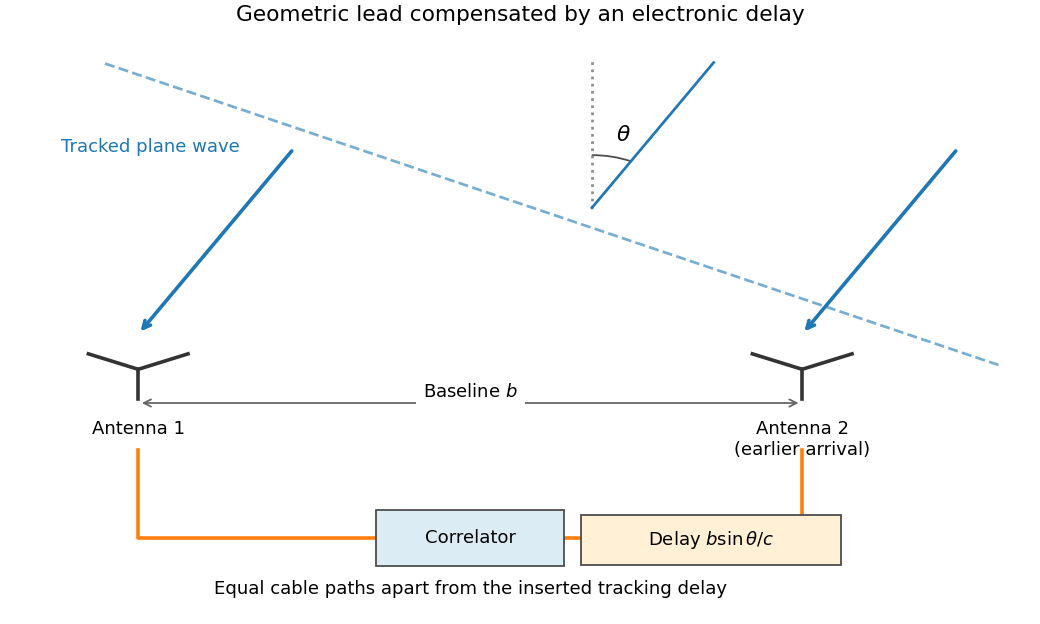
Tracking delay in a two-antenna interferometer
. Original functional schematic. The nearer antenna receives the tracked wave earlier and its electronic delay compensates that geometric lead. Angles are exaggerated and cable paths are schematic. Details.
For a top-hat band centered at , let . Averaging the residual fringe givesAfter removing the central fringe phase, its envelope is exactlyThe full complex average retains the displayed central-frequency phase; the bare sinc in the question is the phase-referenced envelope or an average written in frequency-offset coordinates. This bandwidth decorrelation of a point source is cancellation between different frequency-dependent phases, not absorption of source radiation.
The center-to-center extent is on each side and diagonally, while the shortest nonzero baseline is . At , characteristic scales areThese describe the finest synthesized scale, a largest recoverable scale estimate, and the individual-dish field of view, respectively. Along an array side the longest baseline is only , giving rather than the diagonal estimate. Projection, weighting and sidelobes determine an actual synthesized beam.
There is no sharp universal largest-scale cutoff: the commonly used convention would give . For an ideal uniformly illuminated circular dish, the primary-beam full width at half maximum is approximately , while the first-null angular radius is . These definitions should not be mixed. Uniform lattice spacing also produces grating sidelobes; the primary beam restricts the useful field but does not supply the missing zero-baseline flux.
Use the projected baseline along the source offset, , and . The first bandwidth null occurs at . A worst-case gives . That is a zero of the response, not a good usable bandwidth. A quantitative maximum needs an allowed attenuation.
For example, requiring a response of at least gives at . Hencefor that worst projection. A strictly east-west offset in a sides-aligned square instead samples at most , giving a first null and a ten-percent-loss bandwidth. The original two-antenna geometry supplies an additional projection; these examples use its maximum magnitude. Thus a bandwidth of order is a reasonable conservative estimate with a stated small-loss criterion, rather than a unique geometry-free limit.
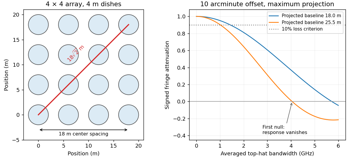
Array baselines and bandwidth decorrelation away from the tracking center
. Original array geometry and rectangular-band sinc calculations for a ten-arcminute offset. The marked ten-percent-loss bandwidth is an illustrative response criterion; the first null is not a usable-bandwidth recommendation. Details.
To use a much wider total band, channelize the signals before correlation or before irreversible frequency averaging. Correlate sufficiently narrow channels, track the reference delay and phase at each frequency, and combine frequency-aware visibilities or images. This preserves sensitivity while avoiding field-dependent averaging losses in radio interferometry. Merely adding a phase correction after a broad channel has decorrelated cannot recover the lost signal; nor can one tracking delay cancel every sky direction simultaneously.[ref]
Field of View by National Radio Astronomy Observatory. VLA Observational Status Summary 2018A, bandwidth and time-averaging limitations
The wavelength corresponds to about , in the low-frequency decrement part of the thermal Sunyaev-Zeldovich effect. Hot cluster electrons inverse-Compton scatter CMB photons. In the Rayleigh-Jeans limit,The signal probes integrated electron pressure. Short baselines give sensitivity to extended arcminute-scale cluster structure, while the primary field covers the cluster and surrounding sky. The array's several-arcminute resolution suits many such structures; it is not equally well matched to every cluster size.
Simultaneous cross-correlations reject uncorrelated receiver noise and provide spatial information; compact radio sources can be constrained with the relatively longer baselines and separated from extended structure. Broad frequency coverage helps sensitivity provided channel smearing is controlled. Correlated atmospheric emission, calibration error, primordial CMB fluctuations and radio-source contamination remain relevant. The lack of zero and very short spacings also means that total integrated cluster flux requires a model or complementary data. An interferometer is therefore useful for the spatially resolved decrement, rather than automatically measuring every cluster's full pressure integral.
An observed catalogue is the result of a population, an instrument and a selection rule. Its astronomical selection function can depend on flux, color, size, surface brightness, sky location, cadence and follow-up success. The relevant cut is often on noisy measured quantities. A model that selects on noiseless true flux instead can predict a different sample even when it uses the same nominal threshold.
Malmquist bias occurs because brighter members of a population are visible through a larger volume in a flux-limited survey. For a uniform Euclidean population, and . The selected luminosity distribution is therefore weighted toward large . For an intrinsic Gaussian absolute-magnitude distribution with mean and variance , multiplying by and completing the square gives the Gaussian absolute-magnitude Malmquist shiftThis assumes the stated simple population, a complete flux cut and no additional boundaries. Exactly identical noiseless standard candles have a distance truncation, not a luminosity spread to reweight. Scatter, extinction, cosmological volume and source evolution need their own model.
Lutz-Kelker bias concerns parallax errors, spatial population weighting and selected calibration samples. Uniform spatial density gives locally, hence on the physically valid range. More distant objects can scatter into a measured-parallax cut. In addition, inversion is nonlinear and gives misleading estimates at low signal-to-noise; a negative measured parallax is possible even for a positive true distance. A posterior instead combines the parallax likelihood with a justified population prior. An unbounded uniform-volume prior is improper here; a finite population model or a proper distance prior for parallax inference is necessary.[ref]
On the Use of Trigonometric Parallaxes for the Calibration of Luminosity Systems: Theory by T. E. Lutz and D. H. Kelker. classical selected-sample parallax-calibration model
Bayes' theorem makes the assumptions explicit. If denotes population parameters, latent properties and the catalogue inclusion event, a selected-sample likelihood has the formThis selection-normalized astronomical likelihood accounts for the model-dependent probability of entering the catalogue. For individual inference, selection information already determined by the fully conditioned measured data must not be multiplied in a second time. The sampling design, inferential target and actual conditioned information determine the appropriate expression.
Other effects include Eddington bias, where steep number counts and measurement scatter move more faint objects upward than bright objects downward, and surface-brightness selection that misses diffuse galaxies despite substantial total flux. Dust extinction affects both detectability and inferred luminosity. Variable-source detection depends on cadence and duration; spectroscopic follow-up can favor easy-to-measure redshifts or particular colors. Blends, calibration drift and redshift errors can mimic population changes.
Examples include magnitude-limited supernova samples used in distance-redshift fits, where luminosity scatter and follow-up must be modeled, and radial-velocity planet surveys, which favor large-amplitude, short-period systems and leave inclination degeneracies. Forward modeling through the survey pipeline, injection-and-recovery estimates of completeness, calibrated noise and properly modeled censored or nondetected observations address these effects. A universal correction or an unexamined inverse-volume weight does not replace an explicit generative and selection model.
Thermal bremsstrahlung arises from electron acceleration in ion Coulomb fields. For a thermal plasma its optically thin spectral emissivity has the dependenceThe exponential high-energy slope helps constrain temperature in X-ray spectra, with composition, absorption and other emission components included. At radio frequencies with , the thin spectrum is much flatter and does not alone determine a unique temperature; the Gaunt factor supplies a weak frequency dependence.
For an approximately isothermal layer, radiative transfer gives . Radio free-free opacity scales approximately as , where the hydrogen-plasma emission measure is . A resolved optically thick brightness temperature approaches ; an unresolved filling factor lowers the observed value. The turnover between thin and thick regimes helps constrain emission measure.
An angular extent and distance give a physical size, and an assumed geometry supplies a line-of-sight depth. Combining that depth with emission measure estimates an rms density, . Clumping, filling factor, composition and unknown depth preserve a density-depth degeneracy of free-free radiation. These measurements constrain different combinations of temperature, density and size rather than independently fixing all three without assumptions.
The radial-velocity method measures repeated Doppler shifts of stellar spectral lines as a star responds to an orbiting companion. A stable high-resolution spectrograph and wavelength reference distinguish stellar motion from instrumental drift; many lines or a spectral template improve precision. A Keplerian fit yields period, eccentricity, phase and velocity semi-amplitude. For a companion mass , stellar mass and inclination ,With a stellar-mass estimate and , this measures approximately , a minimum mass unless the inclination is independently constrained. A nearly face-on orbit can hide a massive companion. The method preferentially detects larger masses, shorter periods and favorable inclinations.
Starspots, activity, pulsations, rotation, blended spectra and sampling aliases can imitate or distort a periodic signal. Line-shape diagnostics, activity indicators, repeated observations and independent constraints help test a planetary explanation. Photon noise and spectral line width constrain precision even for a perfectly calibrated spectrograph. Multiple planets or incomplete orbital coverage require an adequate model and longer monitoring; a periodic centroid shift alone is not a proof of a particular planetary system.
A charge-coupled device converts absorbed photons into stored charge in semiconductor potential wells. An exposure accumulates a pixelated image; clocked electrodes transfer rows toward a serial register and output amplifier. Quantum efficiency, pixel sampling and optical throughput connect collected photons to the expected signal. In ordinary optical imaging it primarily counts photoelectrons rather than independently measuring every photon's energy.
The CCD noise budget combines source and sky shot noise, dark-current fluctuations and read noise. For an aperture containing pixels, known background expectation , total dark expectation , source expectation and per-pixel read noise ,Estimating the background from a finite separate region adds its own uncertainty. Cooling reduces dark current; longer integration reduces the relative importance of one read but can encounter saturation, cosmic rays or changing conditions. Full well capacity, amplifier gain, linearity, blooming and charge-transfer efficiency limit useful detector dynamic range.
Bias frames establish the electronic offset; matched dark frames characterize time- and temperature-dependent dark signal. Flat fields calibrate pixel-to-pixel response and illumination, with appropriate attention to wavelength. Bad-pixel masks, repeated exposures and dithering help reject defects and cosmic rays. A calibrated PSF and astrometric solution are needed for reliable photometry and positions. High quantum efficiency and stable linear integration are advantages, but an uncalibrated count array is not yet an astronomical flux map.
Atmospheric refractive-index fluctuations distort the incoming wavefront. In a Kolmogorov model, the long-exposure seeing width is approximately , where the Fried parameter scales as . High-quality sites and longer wavelengths can improve the observing conditions, but do not eliminate the distorted phase. Short coherence times also require rapid correction or exposure.
Adaptive optics uses a guide source, wavefront sensor, deformable mirror and fast feedback loop. Tip-tilt correction removes image wander; higher-order actuators correct finer spatial distortions. Finite actuator spacing, sensor noise, delay and changing turbulence leave residual errors. A nearby natural guide star limits sky coverage, while a laser beacon supplies higher-order reference information over more directions. Conventional laser-guide-star systems still need independent image-motion information, commonly from a natural star.[ref]
Laser Guide Star for Adaptive Optics by European Southern Observatory. ESO, tip-tilt information and sky-coverage limitation
Anisoplanatism limits the corrected field; laser finite-altitude sampling and variable PSFs need their own calibration.Lucky imaging selects favorable short exposures and aligns them, trading exposure efficiency and photon statistics for reduced blur. Speckle interferometry uses short-exposure spatial-frequency information and suitable phase/statistical reconstruction instead of simply averaging away the speckles. Both need adequate time resolution, detector performance and calibration; selection cannot restore information never recorded. Interferometric methods can also recover fine structure with phase control or closure information. These approaches correct or infer wavefront effects; they do not make clouds, absorption or every atmospheric amplitude fluctuation disappear.[ref]
Adaptive Optics by European Southern Observatory. wavefront sensing, deformable-mirror correction and atmospheric limitations
Articles by others on the same topic
There are currently no matching articles.