Past exam of the general relativity II course of the University of Oxford / 2017 (A12212W1, C7.6)

Source paper: www.whatdotheyknow.com/request/oxford_physics_past_papers_2/response/2340696/attach/5/Physics%20Papers%202016.pdf?cookie_passthrough=1

The coordinate basis vector $K={\partial }_v$ has constant components $K^a={\delta }_v^a$. Its norm isso it is a nonzero null vector everywhere. The Lie derivative of the metric tensor isThus $\boxed{K={\partial }_v\text{ is a null Killing vector field}.}$ In fact it is a parallel vector field: $K_b=g_{bv}={\delta }_b^u$ and the Christoffel symbols found below give ${\nabla }_a{K}_b=-{\Gamma }^u{}_{ab}=0$. This stronger property is characteristic of this plane-fronted gravitational wave.

In the order $(u,v,x,y)$ the metric tensor and inverse metric areOnly $g_{uu}$ has nonzero partial derivatives. Substitution into the formula for the Levi-Civita connection,therefore givesEvery other Christoffel symbol vanishes. For example $g^{ud}$ selects $d=v$, and the metric tensor is independent of $v$ with constant $g_{av}$; hence ${\Gamma }^u{}_{bc}=0$.

Use the paper's Riemann curvature tensor conventionFor the independent components,The quadratic Christoffel symbol terms vanish here: any potentially contributing intermediate $u$ index gives a factor ${\Gamma }^u{}_{ab}=0$, and the remaining possible products have a lower $v$ index and vanish. Since the symmetric matrix $M$ gives $F_{,ij}=2M_{ij}$, lowering the first index givesAll remaining nonzero components follow from the Riemann curvature tensor symmetriesThere are no other independent components: terms involving a $v$ index vanish, while nonzero terms require one $u$ in each antisymmetric pair.

The Ricci tensor is consequentlyThe Ricci scalar vanishes even when the trace is nonzero, since $g^{uu}=0$. With zero cosmological constant, the vacuum Einstein field equations reduce to $R_{ab}=0$. Therefore the necessary and sufficient condition isThis is the Ricci tensor of a Brinkmann plane wave: a nonzero, trace-free profile can have nonzero Riemann curvature tensor despite vanishing Ricci tensor.

The geodesic deviation equation compares neighboring geodesics by covariant derivatives. Replacing those derivatives by ordinary derivatives of coordinate components requires a parallel transport frame along the reference geodesic. There is also an affine parameter normalization to specify: the argument of $M$ is $u$, and it becomes $\tau$ only after choosing $u=\tau$.

For the intended local tidal calculation, take the reference timelike geodesicHere $g(V,V)=-1$, so $\tau$ is proper time. Both $F$ and its first partial derivatives vanish on $\gamma$. All Christoffel symbols therefore vanish along this curve, and its coordinate basis is parallel transport along it. With the Riemann curvature tensor from part (b),The Jacobi field equation thus becomes, in this adapted frame,A purely transverse initial Jacobi field, with ${\sigma }^u={\sigma }^v={\dot{\sigma }}^u={\dot{\sigma }}^v=0$ initially, remains transverse. This transverse tidal equation of a Brinkmann plane wave describes the relative tidal acceleration of the freely falling bodies.

In vacuum write the symmetric matrix asIts instantaneous eigenvalues are $\pm \sqrt{A^2+B^2}$. The tidal acceleration stretches along one principal axis and squeezes along the perpendicular axis, with the axes allowed to vary with $u$. This describes accelerations; it does not imply monotonically growing and shrinking separations for arbitrary initial velocities. For the simple constant profile $A={\omega }^2$, $B=0$,Thus the geodesic deviation can be defocusing in one direction and oscillatory in the other. For a varying profile, diagonalizing at each instant does not decouple the ordinary differential equations without also including derivatives of the rotating eigenvectors.

Qualification of the coordinate claim. The displayed equation for ${\sigma }^v$ is not true for arbitrary coordinate displacements along arbitrary reference geodesics. For synchronized neighboring curves with $u=\tau$ and ${\sigma }^u=0$, the exact geodesic equations areTheir variation givesThe second expression need not vanish. A concrete vacuum counterexample is $M=\mathrm{diag}(1,-1)$ and the one-parameter family of timelike geodesicsEach has $g(V,V)=-1$. Differentiating with respect to $A$ produces a Jacobi fieldThis even has $g(V,\sigma )=0$, so it is a physical orthogonal separation. The covariant derivative form of geodesic deviation remains correct; the unrestricted assertion about ordinary coordinate derivatives needs the adapted reference and frame used above. If instead $\dot{u}=c$ is a constant affine parameter normalization, the transverse tidal coefficient is $c^{2}M(u)$.

Since the real conformal factor $\Lambda$ is nowhere zero, ${\Lambda }^2>0$ at every point. For any tangent vector,The sign is unchanged. With metric signature $(-,+,+,+)$, negative, zero and positive values therefore describe the same timelike vectors, null vectors and spacelike vectors for both metric tensors. In particular the two null cones coincide.

Choose the same time orientation for the two Lorentzian metrics. A future-directed causal curve or timelike curve for one has the same character for the other. Hence the causal future, causal past and chronological future of every point agree:This is the preservation of causal structure by a smooth, nonvanishing conformal transformation. It does not assert preservation of proper time or of affine parameter lengths.

Put $\omega =\log |\Lambda |$, which is smooth because $\Lambda$ is nowhere zero. The conformal change of the Levi-Civita connection isThis follows directly by differentiating ${\tilde{g}}_{ab}=e^{2\omega }{g}_{ab}$ and using ${\tilde{g}}^{ab}=e^{-2\omega }{g}^{ab}$ in the Christoffel symbol formula.

Let $V=dx/d\tau$ be a geodesic tangent for $g$, with $\tau$ an affine parameter. Since ${\nabla }_{V}V=0$,For a null geodesic the second term vanishes. The remaining acceleration is tangent to the same curve and can be removed by changing its parameter. Explicitly set $\tilde{V}=fV$, with $f=d\tau /d\tilde{\tau }$. ThenIt vanishes when $f=C^{-1}{\Lambda }^{-2}$, orThis affine parameter change under conformal rescaling shows that conformal preservation of null geodesic paths means preservation of unparametrized curves; the original affine parameter usually changes.

For a non-null geodesic, the component of ${\mathrm{grad}}_g\omega$ orthogonal to $V$ generally survives. A change of parameter can remove only the tangential component of acceleration. As a concrete example use Minkowski spacetime,The curve $(t,x,y,z)=(\tau ,0,0,0)$ is a timelike geodesic for $g$, but along itThis acceleration is not parallel to ${\partial }_t$, so the curve is not a geodesic of $\tilde{g}$ under any reparametrization. Special non-null curves may still be preserved, for example when $\Lambda$ is constant; nullness is the general guarantee.

The product rule for the Lie derivative and the Killing equation giveConsequently $K$ is a Conformal Killing vector field for the rescaled metric tensor, with smooth conformal Killing factorIt remains an actual Killing vector field precisely when $K(\Lambda )=0$: the conformal factor must be constant along its integral curves of a vector field.

A nondegenerate Lorentzian metric requires $M\ne 0$; take $M>0$ as the radius convention. The original coordinates describe $\lambda >0$, with $\lambda =0$ a candidate boundary rather than an ordinary point of that chart. The change of coordinate givesSubstituting and cancelling the two terms proportional to $d{\lambda }^2/{\lambda }^2$ producesThe $(v,\lambda )$ block of this metric tensor has determinant $-M^2$ and inverse metricAll coefficients are smooth through $\lambda =0$, and the block has one negative and one positive eigenvalue. Together with the positive round two-sphere factor this is a regular Lorentzian metric. It extends to a neighborhood with either sign of $\lambda$. The usual polar-coordinate problem at the poles of the two-sphere is removed by separate angular charts. Therefore $\lambda =0$ is only a coordinate singularity of the original chart. This is the degenerate-horizon patch of Bertotti-Robinson spacetime.

On the extension in part (i), the hypersurface $\mathcal{N}$ has nonzero normal covector $n_a={\partial }_a\lambda$. Its squared norm isThis vanishes on $\mathcal{N}$, which is therefore a null hypersurface. Raising the index givesSince ${\partial }_t={\partial }_v$ at fixed $\lambda$, the original Killing vector field becomes the smooth nonzero field $K={\partial }_v$. The transformed metric tensor is independent of $v$, so $K$ remains a Killing vector field, andThus $K$ is both tangent and normal to $\mathcal{N}$. This is exactly a Killing horizon:The Killing vector field itself does not vanish there; a vanishing squared norm means nullness, not a zero vector.

The Killing equation impliesHere $K^2=-{\lambda }^2$, so in the regular coordinatesThis vector vanishes at $\lambda =0$. The Killing vector field $K={\partial }_v$ is nonzero there, so comparison with the definition of surface gravity yieldsHence this is a degenerate Killing horizon. The argument uses the vanishing gradient of $K^2$ on the horizon; the condition $K^2=0$ by itself would not force zero surface gravity.

A regular hypersurface $f=0$, with $df\ne 0$, is a null hypersurface if its normal covector has zero squared norm:Its normal vector is then also tangent to the hypersurface; the induced metric tensor is degenerate.

For the Kerr metric the normal to a constant-$r$ surface has squared normFor $0<a<M$ the two roots are positive and distinct. To verify that they are genuine regular null hypersurfaces, rather than trusting singular Boyer-Lindquist coordinates, introduce ingoing Kerr coordinatesSubstitution givesThere are no ${\Delta }^{-1}$ terms. At either root $\Sigma >0$, and the determinant is $-{\Sigma }^2{\sin }^2\theta$ away from the angular coordinate poles. Thus the metric tensor extends smoothly across each root. The raised normal on either surface isThis is a nonzero null Killing vector field normal to the surface. Both surfaces are Killing horizons, with horizon angular velocities ${\Omega }_{\pm }$.

The event-horizon terminology in the paper needs qualification. In the usual asymptotically flat Kerr black hole extension, relative to a chosen exterior's future null infinity, the future branch of $r=r_{+}$ is the event horizon, the boundary $\partial J^{-}({\mathcal{I}}^{+})$. In the intervening black-hole region $\Delta <0$, the coordinate $r$ has timelike gradient and future-directed curves move toward smaller $r$; they cannot return across the outer boundary to that exterior. The inner surface $r=r_{-}$ is a Cauchy horizon, not a second event horizon for the same asymptotic end. Nullness is a local property; identifying an event horizon additionally requires this global causal structure.^[ref]

The allowed endpoint $a=0$ provides an especially concrete counterexample to the unrestricted description of both roots. The Kerr metric then becomes Schwarzschild spacetime, $r_{+}=2M$ is its regular event horizon, but $r_{-}=0$ is a curvature singularity:It is not a regular inner null hypersurface. Thus the two-horizon calculation above assumes $0<a<M$.

The metric tensor is independent of $t$ and $\varphi$, soare commuting Killing vector fields. For $0<a<M$ they span the continuous Killing vector field algebra; every constant linear combination is also a Killing vector field. They express stationary spacetime and axial symmetry, respectively. At the allowed endpoint $a=0$ the spherical symmetry of Schwarzschild spacetime enlarges the algebra: in addition to $T$, a basis of rotational Killing vector fields isTheir polar-coordinate expressions are singular at the axis, but the rotational fields are smooth there.

Let $U^a=d{x}^a/ds$ be the tangent to any affinely parametrized geodesic. For a Killing vector field $X$,This is the geodesic conserved quantity from a Killing vector. With $p_a=g_{ab}{U}^b$, choose the energy and axial angular momentum conventionsFor a massive particle with proper time parameter these are per unit rest mass; for a null geodesic their common scale depends on the affine parameter normalization. Expanding in the supplied Boyer-Lindquist coordinates givesThe factor of two between $g_{t\varphi }$ and the coefficient of $dtd\varphi$ is essential for these signs and coefficients.

Reflection across $\theta =\pi /2$ is an isometry; a geodesic initially tangent to its fixed equatorial plane remains in that plane by uniqueness of the geodesic equation. Thus take $\theta =\pi /2$, $\dot{\theta }=0$, and $\Sigma =r^2$. Define the algebraic abbreviationsThe conserved quantities of part (b) becomeFor $\Delta \ne 0$, inversion givesThe null condition can be written without expanding a quadratic square:Substituting the preceding expressions yields the equatorial Kerr null geodesic radial equationAn equivalent useful polynomial form isThese expressions use an affine parameter $s$; a common rescaling of $E$ and $L$ accompanies its rescaling. The inversion was performed in the exterior $r>r_{+}$, where Boyer-Lindquist coordinates are regular. The polynomial radial identity has a smooth continuation to a horizon, but the formulas for $\dot{t}$ and $\dot{\varphi }$ there must be replaced by regular-coordinate expressions. In the limit $a=0$, the result reduces to the Schwarzschild spacetime equation ${\dot{r}}^2=E^2-(1-2M/r)L^2/r^2$.

The assertion about every exterior radius is false for geodesics. A circular orbit here means an equatorial null geodesic at constant $r$, rather than a genuinely radial trajectory. A zero of the radial effective potential alone gives a turning point, not necessarily a circular orbit. The radial geodesic equation must hold as well.

Write $q=L-aE$ andFor an exterior circular null geodesic, the two conditions are $f(r)=f^{\prime }(r)=0$, equivalently $\mathcal{R}(r)={\mathcal{R}}^{\prime }(r)=0$ with $E,L$ fixed. One way to justify the derivative condition without dividing by $\dot{r}=0$ is to use the radial Euler-Lagrange equation. At constant $r$ it givesTogether with $g_{AB}{\dot{x}}^A{\dot{x}}^B=0$, and the fixed conserved $p_A$, this is precisely the double-root condition for $\mathcal{R}$.

NowSetting this to zero and using $f=0$ givesA nontrivial exterior null geodesic cannot have $E=0$ here: the second equation would force $q=L=0$, and then every tangent component would vanish. ThereforeBoth equations, with the same constants $E,L$, are required. They give the requested radius relations in terms of the conserved quantities, while showing why an arbitrary exterior radius is not permitted.

For a more explicit classification let $b=L/E$ be the impact parameter. The second relation gives $b-a=s{r}^{3/2}/\sqrt{M}$ with $s=\pm 1$. Substituting into the first relation yieldsFor $0<a<M$, $s=+1$ gives the prograde equatorial circular Kerr photon orbit and $s=-1$ the retrograde one. The two allowed exterior radii areBoth are strictly greater than $r_{+}$ in the subextremal range. Squaring the signed radius equation gives $r(r-3M{)}^2=4M{a}^2$, but introduces an additional inner root and loses the sign distinguishing the two senses of rotation. At $a=0$ the two exterior radii coincide at the photon sphere $r=3M$, with $b=\pm 3\sqrt{3}M$.

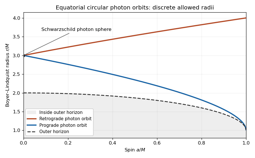
For a direct counterexample to the all-radii claim take $a=0$ and $r_0=4M>r_{+}=2M$. Choose $E=1$ and $L=4\sqrt{2}M$ so that $f(r_0)=0$. The radial geodesic equation nevertheless givesIt is a turning point, not a circular orbit. Alternatively, constant-$r$ null directions exist throughout the exterior because the two angular-velocity roots of $g_{tt}+2\Omega g_{t\varphi }+{\Omega }^2{g}_{\varphi \varphi }=0$ are real; almost all of their integral curves require acceleration and fail the radial geodesic equation. This distinction explains how an all-radii assertion can arise.

Finally, $r=r_{+}$ itself has the null geodesic generators of its Killing horizon, proportional to ${\chi }_{+}={\partial }_v+{\Omega }_{+}{\partial }_{\psi }$. They are a separate horizon case. On the horizon ${\chi }_{+}$ is normal to every tangent, so its contractions with ${\partial }_v$ and ${\partial }_{\psi }$ both vanish: $E=L=0$ for a generator tangent. Its affine parameter can be chosen by rescaling that tangent. The exterior calculation dividing by $E$ does not include it. The presence of these generators does not supply circular null geodesics at the intervening arbitrary exterior radii.