The nonnegative modulus must be a zero of the sine function. The restriction permits , since . Thus the locus is the origin and three concentric circles, centred at the origin with radii , and . A circle of radius zero is just one point.
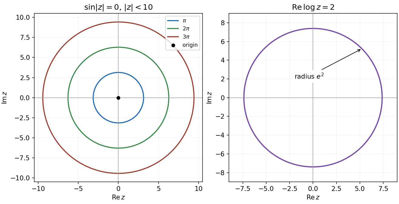
Complex-plane loci: sine of the modulus vanishes on three circles and the origin; real logarithm part fixes one circle
. Details. 
For any value of the complex logarithm, up to adding an integer multiple of . Its real part therefore satisfiesThe locus is the circle centred at the origin with radius . Different logarithm values change only the imaginary part. If a particular analytic branch of the complex logarithm with a cut is imposed, restrict the circle to that branch's domain; the modulus equation itself is branch independent.
The complex sine identity isIt follows either from the exponential definition of sine or its addition formula, using and . ConsequentlyThe angles and in these functions are dimensionless; the real trigonometric argument is measured in radians.
The scalar product fixes the component of the position vector along the given unit normal vector. Thus the locus is a plane normal to , through . Its signed distance from the origin along that normal is , and its perpendicular distance from the origin is . Any displacement lying within the plane is orthogonal to .
Noncoplanarity makes the scalar triple product nonzero, so the three displayed vectors form a reciprocal basis. Their scalar products obeywith all six cross-pairings zero. Therefore, assuming the nonzero needed to define the three given points,Every difference of two of these points is orthogonal to . The two independent differences span their plane, so is a normal to the plane, whose equation is . Also , because its scalar product with each specified point is .
The equations are an eigenvalue problem for the matrixA nonzero solution requires . Expanding givesRow reduction gives the complete eigenspaces:For the solutions form the plane through the origin; for they form a line through the origin. Exclude the zero vector when requiring a nontrivial solution. The repeated eigenvalue has a two-dimensional eigenspace; there are three independent eigenvectors in total. This matrix is not symmetric, so its different eigenspaces need not be mutually orthogonal.
Use direction and displacement . The point-to-line distance is the height of the parallelogram spanned by these vectors:Equivalently the closest line parameter is , giving the foot . Its separation from the point is orthogonal to and has the same length.
Measure the car's vertical displacement from its static equilibrium, so gravity's constant contribution is already balanced. Both the spring and the viscous damper act on motion relative to the wheel. The base-excited oscillator therefore satisfiesFor dimensional clarity write the road profile as ; the printed notation sets the implicit wave number in the chosen length units. Constant forward speed gives forcing angular frequency . With complex amplitudes , the steady response isSet for the expression in the question's notation. Assuming and , the transient response decays, leaving this steady-state response.
For a useful sketch define , and damping ratio . The displacement transmissibility isIt starts at , rises to a finite maximum for finite positive damping, crosses at , then tends to zero. Differentiation with respect to gives the maximum at .
Very small damping permits large resonant oscillations near , producing discomfort and potentially large suspension travel. At exactly zero damping the assumed decay of transients fails, and resonant forcing produces secular growth. Very large damping makes the car follow the bumps over a wide range of speeds, sacrificing vibration isolation: at each fixed forcing frequency, as . For any fixed finite damping the response still eventually decreases at sufficiently high frequency. These two limits should not be interchanged.
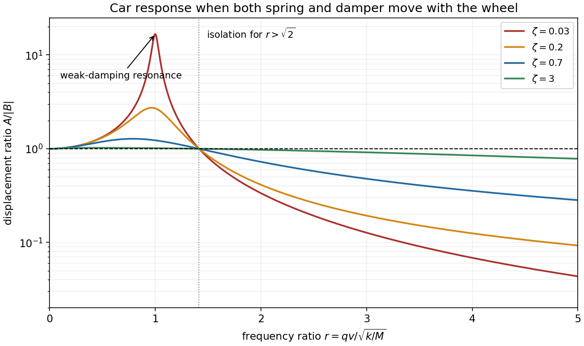
Base-excited car displacement response for several damping ratios, including the weak-damping resonance and isolation threshold
. Details. 
Split the mixed quadratic terms evenly across a real symmetric matrix:Its characteristic polynomial isso . Choose the orthonormal eigenvectorsThe orthogonal transformation givesIndeed and ; preserving is precisely the length-preserving property of an orthogonal matrix.
The requested plane has normal . An orthonormal basis within it isWrite a point of that plane as . Restricting the quadratic form gives , so its section with isIt is an ellipse centred at the origin, with semi-axes along and along . Normalizing the in-plane basis is essential: coefficients in nonorthonormal coordinates would not directly give physical lengths.
The complete surface is the one-sheet hyperboloidIt is connected, extends indefinitely in both directions along its axis , and has an elliptical waist at with semi-axes and . At larger its transverse sections widen; its asymptotic cone is . The specified plane is oblique to that axis, rather than the waist plane.
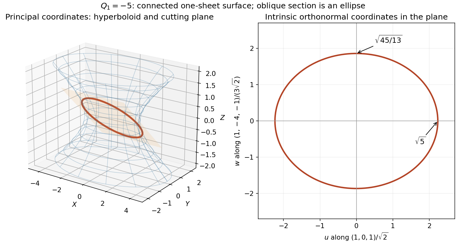
One-sheet hyperboloid in principal coordinates and its oblique elliptical section, with the intrinsic semi-axis lengths
. Details. 
For , the integrating factor for can be taken as on either half-line. Thus , givingThe arbitrary constant may differ on the disconnected domains and .
The initial point lies in , where division by is valid. The first-order linear differential equationhas integrating factor . HenceThe condition at sets , soThe solution cannot be continued regularly through : its numerator tends to while the denominator tends to zero. The real logarithm also requires .
The characteristic equation of the homogeneous ordinary differential equation is , with roots . Therefore . For the forcing term, try the particular solution . Substitution gives , , so , . The two initial conditions give and . ConsequentlyBoth the value and the first derivative vanish at zero; direct differentiation verifies the inhomogeneous equation.
For the Cauchy-Euler equation , the power trial on gives . The repeated root supplies the logarithmic second solution. On either half-line,One may also obtain this by setting , which reduces the equation to . Constants on opposite sides of the singular point need not agree.
Expanding and equating coefficients gives , . ThusThe two-argument arctangent fixes the quadrant; if , the phase is arbitrary.
For the coupled ordinary differential equations, set . The first equation becomes , and the initial values give . The second then reduces to . Its initial value problem has solutionWhere , reconstruct . The scalar function is smooth for every real , but the original coupled system cannot have a finite at its first zero, about . The requested sketch up to can display the analytic continuation of , with that distinction marked. Initially , and ; it first rises, reaches a maximum, then decreases through zero and becomes negative within the plotted interval.
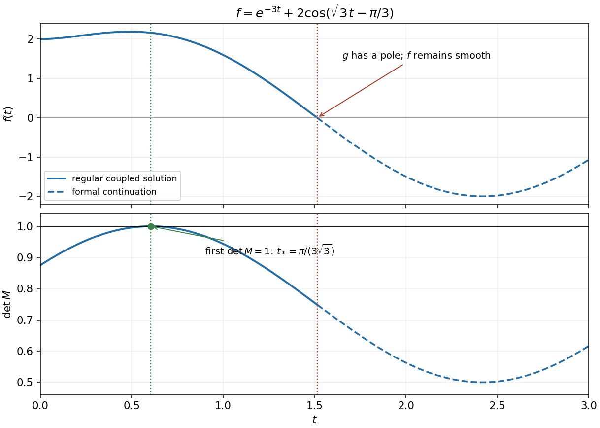
The scalar solution and matrix determinant, with the first regular rotation time and the later pole in the reconstructed variable
. Details. 
For the determinant of , separate its upper-left block from the constant last diagonal entry. Using givesThus precisely when . The smallest positive solution isIt occurs before the zero of , so and are finite there. Put . At this time the upper block isFor a rotation matrix, each column must have unit norm, giving . Both signs are allowed by the stated assumption that is a constant:Both have determinant and preserve lengths. If a positive is intended, only the first row remains; positivity is not stated in the question.
The transpose of a matrix product reverses factor order:For the requested two-dimensional check, put and . Both sides areMore generally, the entry formula is exactly .
The conjugate transpose also reverses factor order. If and are unitary matrices,Thus their product is unitary. This is closure under multiplication in the unitary group.
For a Hermitian matrix , . Reversing the product of identical factors has no effect, soHence every positive integer power is Hermitian. The identical-factor condition matters; a product of different Hermitian matrices need not be Hermitian.
At the power series gives . Equate the coefficient of after differentiating the series and substituting into the linear system of ordinary differential equations:Mathematical induction yields . Summing gives the matrix exponential solution .
For the specified diagonal Hermitian matrix, its powers and exponential act separately on the two components. ThusThis unitary matrix preserves : the two components acquire opposite phases of unit modulus. The coefficient recurrence applies to any constant finite square matrix ; unitarity here additionally uses its Hermitian property.
Articles by others on the same topic
There are currently no matching articles.