Past exam of the mathematical models of financial derivatives course of the University of Oxford / 2023 (B8.3, A13374W1)

Source: released examination PDF, pages 252–255. Solutions follow the numbering of the 6 June 2023 paper. Throughout, volatility is positive and the stated Black-Scholes model assumptions apply. The finite perpetual values in 2(b) additionally require $r>0$; the other interest-rate cases are explained below. Question 3's conditional expectation is evaluated under the measure stipulated there, with its financial interpretation qualified in 3(d).

Use a self-financing portfolio which holds $\Delta =V_S$ shares and $V-S{V}_S$ in the bank account, withdrawing the claim's cash flow $Cdt$. A share's total gain includes the continuous dividend yield, so its gain is $dS+DSdt$. Matching the claim's total gain givesBy the Itô formula,The delta hedge cancels the Brownian motion term. Comparing the remaining drifts yields the Black-Scholes equation with claim dividends, with the stock's own dividend yield included:This gain calculation accounts for rebalancing through the self-financing portfolio condition. The physical expected-return parameter $\mu$ cancels, as required by risk-neutral pricing.

For claim dividends proportional to the underlying stock, put $V(S,t)=S\varphi (t)$. Then $V_S=\varphi$, $V_{SS}=0$ and $V_t=S{\varphi }^{\prime }$, so the partial differential equation reduces to the linear ordinary differential equationThe integrating factor $e^{-Dt}$ gives $(e^{-Dt}\varphi {)}^{\prime }=-e^{-Dt}f(t)$. Integrating backwards from the terminal value,The formula assumes the displayed integral is finite. Under the risk-neutral measure, ${\mathbb{E}}_t[S_u]=S{e}^{(r-D)(u-t)}$. Discounting each cash payment at its own payment time gives the same result:The interest rate disappears because every payment is proportional to the stock price.

Setting $f=0$ in b givesThis is a prepaid forward contract: the holder pays now and receives one share at $T$, with no interim dividend payments. Buying $e^{-D(T-t)}$ shares now and reinvesting their continuous dividend yield grows the shareholding to one at expiry. Thus the displayed initial cost replicates the terminal delivery. When $D=0$, holding one share already does so and $V=S$.

For the non-dividend-paying stock, a self-financing portfolio replicating a smooth European option has $\Delta =V_S$ shares and $V-S{V}_S$ in the bank account. Its gain satisfiesThe Itô formula gives $dV=(V_t+\mu S{V}_S+{\sigma }^2{S}^2{V}_{SS}/2)dt+\sigma S{V}_{S}dW$. Matching its diffusion and drift with the portfolio gains cancels $\mu$, yieldingThe financial payoff supplies the terminal value. This is the Black-Scholes equation; the associated risk-neutral measure replaces the physical stock drift by $r$.

Write $\tau =T-t>0$ and $g_n(s)=(K-s{)}_{+}^n$. The European power put formula isHere $Y>0$ has a lognormal distribution. Since $g_n$ is decreasing and is a convex function, its discounted expected value is also decreasing and convex as a function of $S$. For $S>0$ it is smooth and strictly positive: the normal distribution assigns positive probability to $SY<K$ whatever the current positive spot price. Its endpoints areThe dominated convergence theorem justifies the second limit, because $0\le (K-SY{)}_{+}^n\le K^n$. For a quantitative sketch, the binomial theorem and truncated lognormal moment givewhere $\Phi$ is the standard normal distribution function. This finite sum is useful for drawing the curve; its positive expectation form makes its qualitative shape clearer.

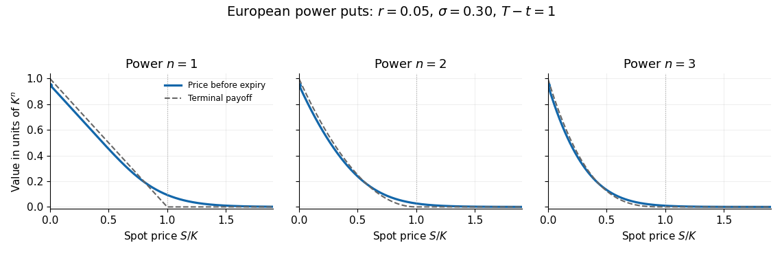
The solid curves use $K=1$, $r=0.05$, $\sigma =0.30$ and $\tau =1$; the dashed curves show their terminal financial payoffs for comparison. Each price remains positive at $S=K$ and tends smoothly towards zero beyond it. At small $S$, discounting gives a price below the undiscounted financial payoff; European exercise is permitted only at expiry.

Assume $r>0$, put $b=S^{\star }\in (0,K)$ and let ${\tau }_b=\inf \{u\ge 0:S_u\le b\}$. In the continuation region $S>b$, the time-independent Black-Scholes equation is a Cauchy-Euler equation. Substituting $V=S^m$ givesSet $\gamma =2r/{\sigma }^2>0$. The two powers are $S$ and $S^{-\gamma }$. The boundary condition $V(S)\to 0$ as $S\to \infty$ removes the growing solution; value matching at $b$ sets the coefficient. Hence the fixed-trigger value isFor $0\le S\le b$ the policy exercises immediately, giving $V_b(S)=(K-S{)}^n$. The quoted continuation expression alone does not apply below the exercise boundary. Equivalently, the discounted boundary-hitting representation gives ${\mathbb{E}}_S[e^{-r{\tau }_b};{\tau }_b<\infty ]=(S/b{)}^{-\gamma }$, which multiplies the exercise financial payoff.

For $S>b$, maximize the coefficient $H(b)=b^{\gamma }(K-b{)}^n$ of $S^{-\gamma }$. Its logarithmic derivative isIt changes sign once, at $b=\gamma K/(\gamma +n)$. The perpetual power put option therefore has candidate valueThe same boundary follows from smooth fit, $-\gamma (K-b{)}^n/b=-n(K-b{)}^{n-1}$. To establish optimality among all stopping times, rather than only fixed barriers, we verify the candidate. Let $\mathcal{L}=rS{\partial }_S+{\sigma }^2{S}^2{\partial }_{SS}/2$ be the infinitesimal generator. The maximum property of $H$ gives $V_n\ge g_n$ everywhere, and $(\mathcal{L}-r)V_n=0$ for $S>b$. For $S\le b$, set $y=S/(K-S)\le \gamma /n$. ThenThus the discounted candidate is a nonnegative supermartingale. The smooth fit removes the derivative-jump local time of a semimartingale term in the Itô formula. The optional stopping theorem and localization bound every exercise policy's discounted expected value by $V_n$. Immediate exercise attains it below $b$; the first hitting time of $b$ attains it above $b$. The terminal remainder vanishes since $0\le e^{-ru}{V}_n(S_u)\le K^n{e}^{-ru}\to 0$. This proves the displayed value.

For $n=1$ it reduces to the ordinary perpetual put option. Larger $n$ lowers the optimal trigger, because the more strongly curved financial payoff makes further downward moves more valuable. If $r=0$, under the risk-neutral measure the stock tends to zero almost surely, so the supremum is $K^n$, approached as the exercise time tends to infinity and not attained at a finite time when $S>0$. If $r<0$, the values at deterministic exercise times grow without bound; the perpetual value is infinite. These cases do not admit the positive-rate formula above.

For $x_t=\log S_t$, the Itô formula uses $(\log S{)}^{\prime }=1/S$ and $(\log S{)}^{\prime \prime }=-1/S^2$. ConsequentlyThe quadratic variation term shifts the mean level. Thus the log-mean-reverting price has logarithm following the Ornstein-Uhlenbeck processIt is the logarithm, rather than the price itself, which reverts linearly to a constant mean level.

Apply the Itô product rule with deterministic integrating factor $e^{\alpha u}$:Integrate from $t$ to $T$ and multiply by $e^{-\alpha T}$ to obtainThis is the explicit solution behind the Ornstein-Uhlenbeck transition distribution.

Write $\tau =T-t$ and $a=e^{-\alpha \tau }$. The stochastic integral in b has a deterministic integrand, so it is a Gaussian random variable independent of the information available at $t$. Its variance, by the Itô isometry, isThus $x_T$ conditionally has a normal distribution with expected value $m=a{x}_t+(1-a)\tilde{\mu }$ and variance $v$. The moment-generating function of a normal distribution gives ${\mathbb{E}}_t[e^{x_T}]=e^{m+v/2}$, so the conditional mean of a log-mean-reverting price isThe correction $v/2$ is essential: exponentiating the conditional mean of the logarithm alone would omit the dispersion of the lognormal distribution.

Keep the maturity $T$ fixed and write $F(t,T)=\exp L(t,x_t)$, whereAs calendar time increases, ${\partial }_{t}a=\alpha a$, so $L_x=a$, $L_{xx}=0$ and $L_t=\alpha a(x-\tilde{\mu })-{\sigma }^2{a}^2/2$. Applying the Itô formula to $L$ and then to its exponential givesThe Itô formula's exponential correction cancels the displayed drift of $L$. The zero drift also follows from the tower property of conditional expectation: for $t\le u\le T$, ${\mathbb{E}}_t[F(u,T)]={\mathbb{E}}_t[S_T]=F(t,T)$. In particular $F(T,T)=S_T$, while the quote's instantaneous spot volatility approaches $\sigma$ as expiry approaches.

This is a martingale under the same measure used in the stipulated conditional expectation. To interpret it as futures pricing, that measure must be a suitable pricing measure. For a non-dividend-paying traded stock at a deterministic interest rate, the absence of arbitrage instead gives a forward contract delivery price $S_t{e}^{r(T-t)}$. A physical-measure expectation under the given mean-reverting drift is not automatically that price; the question's expectation convention is sufficient for the calculation above, but not for this additional identification.