Mathematical models of financial derivatives course of the University of Oxford (B8.3)

Source: released examination PDF, pages 252–255. Solutions follow the numbering of the 6 June 2023 paper. Throughout, volatility is positive and the stated Black-Scholes model assumptions apply. The finite perpetual values in 2(b) additionally require $r>0$; the other interest-rate cases are explained below. Question 3's conditional expectation is evaluated under the measure stipulated there, with its financial interpretation qualified in 3(d).

Use a self-financing portfolio which holds $\Delta =V_S$ shares and $V-S{V}_S$ in the bank account, withdrawing the claim's cash flow $Cdt$. A share's total gain includes the continuous dividend yield, so its gain is $dS+DSdt$. Matching the claim's total gain givesBy the Itô formula,The delta hedge cancels the Brownian motion term. Comparing the remaining drifts yields the Black-Scholes equation with claim dividends, with the stock's own dividend yield included:This gain calculation accounts for rebalancing through the self-financing portfolio condition. The physical expected-return parameter $\mu$ cancels, as required by risk-neutral pricing.

For claim dividends proportional to the underlying stock, put $V(S,t)=S\varphi (t)$. Then $V_S=\varphi$, $V_{SS}=0$ and $V_t=S{\varphi }^{\prime }$, so the partial differential equation reduces to the linear ordinary differential equationThe integrating factor $e^{-Dt}$ gives $(e^{-Dt}\varphi {)}^{\prime }=-e^{-Dt}f(t)$. Integrating backwards from the terminal value,The formula assumes the displayed integral is finite. Under the risk-neutral measure, ${\mathbb{E}}_t[S_u]=S{e}^{(r-D)(u-t)}$. Discounting each cash payment at its own payment time gives the same result:The interest rate disappears because every payment is proportional to the stock price.

Setting $f=0$ in b givesThis is a prepaid forward contract: the holder pays now and receives one share at $T$, with no interim dividend payments. Buying $e^{-D(T-t)}$ shares now and reinvesting their continuous dividend yield grows the shareholding to one at expiry. Thus the displayed initial cost replicates the terminal delivery. When $D=0$, holding one share already does so and $V=S$.

For the non-dividend-paying stock, a self-financing portfolio replicating a smooth European option has $\Delta =V_S$ shares and $V-S{V}_S$ in the bank account. Its gain satisfiesThe Itô formula gives $dV=(V_t+\mu S{V}_S+{\sigma }^2{S}^2{V}_{SS}/2)dt+\sigma S{V}_{S}dW$. Matching its diffusion and drift with the portfolio gains cancels $\mu$, yieldingThe financial payoff supplies the terminal value. This is the Black-Scholes equation; the associated risk-neutral measure replaces the physical stock drift by $r$.

Write $\tau =T-t>0$ and $g_n(s)=(K-s{)}_{+}^n$. The European power put formula isHere $Y>0$ has a lognormal distribution. Since $g_n$ is decreasing and is a convex function, its discounted expected value is also decreasing and convex as a function of $S$. For $S>0$ it is smooth and strictly positive: the normal distribution assigns positive probability to $SY<K$ whatever the current positive spot price. Its endpoints areThe dominated convergence theorem justifies the second limit, because $0\le (K-SY{)}_{+}^n\le K^n$. For a quantitative sketch, the binomial theorem and truncated lognormal moment givewhere $\Phi$ is the standard normal distribution function. This finite sum is useful for drawing the curve; its positive expectation form makes its qualitative shape clearer.

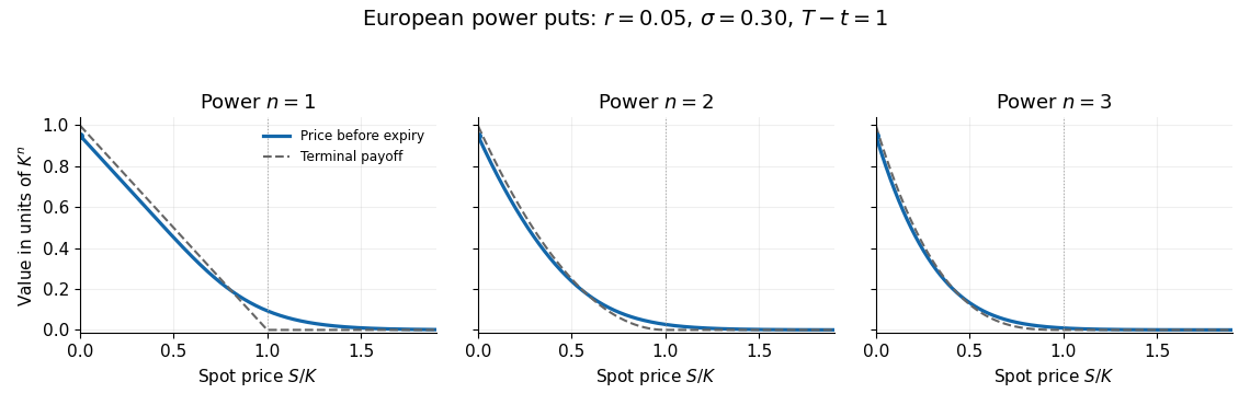
The solid curves use $K=1$, $r=0.05$, $\sigma =0.30$ and $\tau =1$; the dashed curves show their terminal financial payoffs for comparison. Each price remains positive at $S=K$ and tends smoothly towards zero beyond it. At small $S$, discounting gives a price below the undiscounted financial payoff; European exercise is permitted only at expiry.

Assume $r>0$, put $b=S^{\star }\in (0,K)$ and let ${\tau }_b=\inf \{u\ge 0:S_u\le b\}$. In the continuation region $S>b$, the time-independent Black-Scholes equation is a Cauchy-Euler equation. Substituting $V=S^m$ givesSet $\gamma =2r/{\sigma }^2>0$. The two powers are $S$ and $S^{-\gamma }$. The boundary condition $V(S)\to 0$ as $S\to \infty$ removes the growing solution; value matching at $b$ sets the coefficient. Hence the fixed-trigger value isFor $0\le S\le b$ the policy exercises immediately, giving $V_b(S)=(K-S{)}^n$. The quoted continuation expression alone does not apply below the exercise boundary. Equivalently, the discounted boundary-hitting representation gives ${\mathbb{E}}_S[e^{-r{\tau }_b};{\tau }_b<\infty ]=(S/b{)}^{-\gamma }$, which multiplies the exercise financial payoff.

For $S>b$, maximize the coefficient $H(b)=b^{\gamma }(K-b{)}^n$ of $S^{-\gamma }$. Its logarithmic derivative isIt changes sign once, at $b=\gamma K/(\gamma +n)$. The perpetual power put option therefore has candidate valueThe same boundary follows from smooth fit, $-\gamma (K-b{)}^n/b=-n(K-b{)}^{n-1}$. To establish optimality among all stopping times, rather than only fixed barriers, we verify the candidate. Let $\mathcal{L}=rS{\partial }_S+{\sigma }^2{S}^2{\partial }_{SS}/2$ be the infinitesimal generator. The maximum property of $H$ gives $V_n\ge g_n$ everywhere, and $(\mathcal{L}-r)V_n=0$ for $S>b$. For $S\le b$, set $y=S/(K-S)\le \gamma /n$. ThenThus the discounted candidate is a nonnegative supermartingale. The smooth fit removes the derivative-jump local time of a semimartingale term in the Itô formula. The optional stopping theorem and localization bound every exercise policy's discounted expected value by $V_n$. Immediate exercise attains it below $b$; the first hitting time of $b$ attains it above $b$. The terminal remainder vanishes since $0\le e^{-ru}{V}_n(S_u)\le K^n{e}^{-ru}\to 0$. This proves the displayed value.

For $n=1$ it reduces to the ordinary perpetual put option. Larger $n$ lowers the optimal trigger, because the more strongly curved financial payoff makes further downward moves more valuable. If $r=0$, under the risk-neutral measure the stock tends to zero almost surely, so the supremum is $K^n$, approached as the exercise time tends to infinity and not attained at a finite time when $S>0$. If $r<0$, the values at deterministic exercise times grow without bound; the perpetual value is infinite. These cases do not admit the positive-rate formula above.

For $x_t=\log S_t$, the Itô formula uses $(\log S{)}^{\prime }=1/S$ and $(\log S{)}^{\prime \prime }=-1/S^2$. ConsequentlyThe quadratic variation term shifts the mean level. Thus the log-mean-reverting price has logarithm following the Ornstein-Uhlenbeck processIt is the logarithm, rather than the price itself, which reverts linearly to a constant mean level.

Apply the Itô product rule with deterministic integrating factor $e^{\alpha u}$:Integrate from $t$ to $T$ and multiply by $e^{-\alpha T}$ to obtainThis is the explicit solution behind the Ornstein-Uhlenbeck transition distribution.

Write $\tau =T-t$ and $a=e^{-\alpha \tau }$. The stochastic integral in b has a deterministic integrand, so it is a Gaussian random variable independent of the information available at $t$. Its variance, by the Itô isometry, isThus $x_T$ conditionally has a normal distribution with expected value $m=a{x}_t+(1-a)\tilde{\mu }$ and variance $v$. The moment-generating function of a normal distribution gives ${\mathbb{E}}_t[e^{x_T}]=e^{m+v/2}$, so the conditional mean of a log-mean-reverting price isThe correction $v/2$ is essential: exponentiating the conditional mean of the logarithm alone would omit the dispersion of the lognormal distribution.

Keep the maturity $T$ fixed and write $F(t,T)=\exp L(t,x_t)$, whereAs calendar time increases, ${\partial }_{t}a=\alpha a$, so $L_x=a$, $L_{xx}=0$ and $L_t=\alpha a(x-\tilde{\mu })-{\sigma }^2{a}^2/2$. Applying the Itô formula to $L$ and then to its exponential givesThe Itô formula's exponential correction cancels the displayed drift of $L$. The zero drift also follows from the tower property of conditional expectation: for $t\le u\le T$, ${\mathbb{E}}_t[F(u,T)]={\mathbb{E}}_t[S_T]=F(t,T)$. In particular $F(T,T)=S_T$, while the quote's instantaneous spot volatility approaches $\sigma$ as expiry approaches.

This is a martingale under the same measure used in the stipulated conditional expectation. To interpret it as futures pricing, that measure must be a suitable pricing measure. For a non-dividend-paying traded stock at a deterministic interest rate, the absence of arbitrage instead gives a forward contract delivery price $S_t{e}^{r(T-t)}$. A physical-measure expectation under the given mean-reverting drift is not automatically that price; the question's expectation convention is sufficient for the calculation above, but not for this additional identification.

Source: original released examination PDF, bundle pages 66–69; paper pages 1–4. The bundle filename says 2020, but the printed paper is dated 2 June 2021.

Solutions to all three questions. Write $\tau =T-t$, $\Phi$ for the standard normal distribution function, and $\varphi$ for the standard normal density. Formulas with $\tau$ in a denominator are for $t<T$; terminal values are specified separately. Barrier formulas refer to a contract whose barrier has not previously been hit, unless stated otherwise.

The portfolio value is ${\Pi }_t={\varphi }_t{S}_t+{\psi }_t{B}_t$. The self-financing condition means that changes in holdings are financed by trading within the portfolio, with no external infusion or withdrawal. ThusThe holdings are predictable and satisfy the usual stochastic-integrability and admissibility conditions; without admissibility, doubling strategies would spoil the intended no-arbitrage interpretation.

For $V\in C^{1,2}$, Itô's formula givesMatch the Brownian coefficient with the self-financing portfolio by choosing the option delta $\varphi =V_s$ and bond value $\psi B=V-s{V}_s$. Equating drifts cancels the physical drift $\mu$ and givesThis is the pricing equation for a linear asset with additive noise. Its spatial domain is the whole real line, because the asset can be negative. In particular the diffusion term is ${\sigma }^2{V}_{ss}/2$, not ${\sigma }^2{s}^2{V}_{ss}/2$. The derivation is delta hedging and does not impose a boundary condition at $s=0$.

Set ${\theta }_t=(\mu -r)S_t/\sigma$. The Girsanov theorem uses the densityFor these nonexplosive linear stochastic differential equations, the linear drift change of measure ensures that $Z$ is a true martingale on each finite horizon. This matters: a stochastic exponential being a local martingale alone would not prove that its terminal expectation is one. Its strict positivity gives an equivalent risk-neutral measure $\mathbb{Q}$, under whichThe discounted asset is then a martingale. The Feynman-Kac formula, equivalently risk-neutral valuation of the replicable claim, givesHere the payoff must meet the usual integrability and replication assumptions; the bounded digital payoff below does.

The discounted stock over the remaining horizon satisfiesThe Itô integral on the right is a centered normal random variable with variance $a_{\tau }=(1-e^{-2r\tau })/(2r)$. Therefore $\mathbb{Q}(S_T\ge 0\mid S_t=s)=\Phi (d)$, where $d=s/(\sigma \sqrt{a_{\tau }})$. The digital option price and its option delta areThe formula also shows $V(t,0)=e^{-r\tau }/2$ for every $t<T$. At maturity use the specified step payoff, including its chosen value one at zero; the terminal discontinuity is not removed by the earlier-time smoothing.

Since $a_{\tau }$ does not depend on $\sigma$, differentiation of the digital option value gives its vega:Thus vega is negative for $s>0$, zero at $s=0$, and positive for $s<0$. Increasing volatility spreads the conditional normal distribution around its mean: when the current asset value is positive this reduces the chance of ending positive, while for a negative starting value it increases that chance. At zero the distribution stays symmetric and the probability remains one half. A digital payoff need not have the positive vega familiar from a European call option.

A self-financing replicating portfolio for a terminal payoff $F(S_T)$ has the same terminal value on every relevant path, with all earlier rebalancing funded internally. In a complete market its initial cost is unique under no-arbitrage: otherwise buy the cheaper payoff and sell the more expensive identical payoff.

In the Black-Scholes model, the portfolio holds $V_s$ shares and bond value $V-S{V}_s$, where $V$ solves the Black-Scholes equation with terminal data $F$. Itô's formula verifies the self-financing condition. Equivalently,This relates claim replication, the Black-Scholes equation, and risk-neutral valuation.

Buy $1/F_0^T$ shares and take a short forward contract for $1/F_0^T$ shares at delivery price $F_0^T$. The forward has zero initial value, and the combined terminal payoff isTherefore the synthetic zero-coupon bond has initial priceIts implied continuously compounded maturity yield is $r_T=T^{-1}\log (F_0^T/S_0)>0$.

To replicate a constant-rate risk-free asset throughout the interval, the market must support dynamically coherent discounting, not just this one terminal payment. A sufficient condition is that for all $0\le t\le u\le T$ the fair forward prices satisfy $F_t^u=S_t{e}^{r(u-t)}$ for the same deterministic $r>0$, with the required stock/forward positions tradable and no intervening payments. Then $P(t,u)=S_t/F_t^u=e^{-r(u-t)}$, and a suitably scaled fixed-maturity zero-coupon bond grows deterministically as $e^{rt}$. A single initial forward quote does not establish these intermediate-time conditions; even a flat initial yield curve need not imply deterministic future rates.

Under the risk-neutral measure, writeComplete the square in the normal density after multiplying by the power of $S_T/s$. The truncated lognormal moment gives, for $K>0$,All real powers have finite moments in this lognormal distribution. If $K=0$, the indicator is identically one and $V_p=M_p$. The function $V_p$ is an undiscounted conditional moment; the option prices below additionally include the discount factor.

If $p>0$ and $K>0$, the payoff is positive exactly when $S_T>k:=K^{1/p}$. Splitting it into two truncated moments givesFor $p=0$, the payoff is the constant $(1-K{)}^{+}$, so its price is $e^{-r\tau }(1-K{)}^{+}$. For $K=0$ and $p>0$, its price is $e^{-r\tau }{s}^p{M}_p(\tau )$. These boundary cases avoid taking $K^{1/p}$ when $p=0$.

The payoff is $(S_0{S}_T-S_T^2)1_{\{S_T<S_0\}}$. Subtract the upper-tail truncated lognormal moments from the full moments in part c. With current spot $s=S_t$, the price iswhere $M_1=e^{r\tau }$ and $M_2=e^{(2r+{\sigma }^2)\tau }$. The threshold is the original $S_0$, not the current spot $s$. Since the conditional lognormal distribution has no atoms, the strict endpoint convention does not affect the price for $t<T$.

The logarithm of the geometric average isBy stochastic Fubini theorem, ${\int }_0^T{W}_{u}du={\int }_0^T(T-v)d{W}_v$, a centered Gaussian random variable with variance $T^3/3$. ThereforeThe Geometric Asian option is consequently a call on this lognormal random variable. Completing the square as in part c givesThe averaging changes both the log-mean and log-variance; replacing $S_T$ by an ordinary stock price at a shorter maturity without these adjustments would give the wrong formula.

For a long position in the claim, hold $-V_S$ shares and bank value $S{V}_S-V$ so that claim plus hedge has zero initial value. The Black-Scholes equation and Itô's formula show that the total position is self-financing and its Brownian and drift terms cancel. Equivalently, the positive replicating portfolio holds $V_S$ shares and bond value $V-S{V}_S$.

Under the usual growth, integrability and admissibility conditions, no-arbitrage forces the claim price to be $V$: a different price could be traded against the replicating portfolio. The qualification matters because an arbitrary formal PDE solution without a suitable financial class need not be a valid price.

Let ${\tau }_B=\inf \{u\ge t:S_u\le B\}$. While the contract is alive, the down-and-out put pays $(K-S_T{)}^{+}{1}_{\{{\tau }_B>T\}}$ at maturity; a prior touch has already knocked it out.

The truncated terminal payoff can be represented by the ordinary European-price combinationAt maturity its three regions areIndeed it is zero below $B$, equals $K-S$ between $B$ and $K$, and is zero above $K$. This supplies the terminal building block for reflection.

The zero-below-barrier property is a property of the terminal payoff. Before maturity, $F(S,t)$ need not vanish for $S<B$, because the ordinary European contracts can still finish above $B$. The killed barrier option price, rather than this unrestricted European combination, is zero after a touch.

Put $q=1-2r/{\sigma }^2$. The Black-Scholes reflection symmetry maps $F$ to $(S/B{)}^{q}F(B^2/S,t)$, which solves the same PDE. Their difference vanishes at $S=B$. For $S>B$ at maturity the reflected argument is below $B$, where the terminal function in part ii is zero. Thus the boundary and terminal data of the alive down-and-out put are satisfied:The killed-domain Feynman-Kac formula identifies this solution with the discounted payoff conditional on survival. For $S\le B$, or after any prior barrier hit, the actual price is zero. The reflected difference is a formula on the alive domain $S>B$; extending that algebraic expression to $S<B$ generally gives a nonzero, possibly negative function and is not a valid barrier-option price.

A down-and-out digital call with strike at the barrier pays one exactly when the barrier is avoided until expiry. Reflection therefore gives its alive priceThe complementary contract pays one at expiry when the barrier has been hit. Its price isThis is a cash-at-expiry one-touch option, not cash paid at the first touch. After the barrier has already been hit, its price is $e^{-r\tau }$ regardless of the current spot. In particular this branch applies immediately for $S\le B$. Current spot alone does not encode the full path history.

If the barrier is reached, path continuity gives $S_{{\tau }_B}=B$ and the early payment is $K-B$. If it is not reached, the terminal payment is exactly the down-and-out put payoff. When $r=0$, moving a fixed payment from the hitting time to expiry does not change its value. Hence the barrier-triggered put price isHere $G,H$ are evaluated with zero interest rate. If the barrier has already been hit, the exploding put has been exercised and has no remaining value after its payment; the displayed replication concerns an initially alive contract and its cash flows.

The barrier-triggered put exercises at the particular stopping time ${\tau }_B\wedge T$. The American put option optimizes over all allowed exercise times, soIt can be strictly smaller, but can never exceed the American value. Equality is possible if immediate exercise is already triggered and optimal; a fixed barrier is not generally the optimal finite-maturity exercise rule.

The comparison with the European put option can go in either direction. By the early exercise premium for a fixed barrier,Thus an early payment gains interest but sacrifices remaining put time value; the expression inside braces need not have a fixed sign for arbitrary barriers.

For a concrete general construction take current spot $S\ge K$, $r>0$, $\sigma >0$, and $t<T$. Set $\gamma =2r/{\sigma }^2$ and $b_{\infty }=K\gamma /(1+\gamma )$, the perpetual put option exercise boundary. For $0<B<b_{\infty }$, the perpetual value at $B$ equals $K-B$ and strictly dominates the finite-maturity European value. The premium formula and positive probability of hitting $B$ therefore give $E_B>P$. Strictness follows from the perpetual verification argument: before a fixed positive expiry, its discounted value loses drift $rK$ whenever the stock is below $b_{\infty }$, with positive expected occupation time when started at $B<b_{\infty }$.

Conversely, for $B<K$ sufficiently close to $K$, every possible payment of the exploding put is at most $K-B$, whether paid at touch or on surviving to expiry. Hence $0\le E_B\le K-B\to 0$, while $P(S,t;K)>0$. This gives $E_B<P$ for such barriers, and also strict inequality below the American value.

These examples establish both possibilities in general, not a claim that every fixed initial state admits both. If $S<b_{\infty }$ and only alive barriers $B<S$ are allowed, all those barriers are in the same perpetual stopping region and the premium comparison is nonnegative.

Source: released examination PDF, bundle pages 63–66.

Solutions to all three questions and all optional parts. Expectations in Question 1 are conditional on current information. The zero-drift variance is obtained by a limit. The exercise-policy calculation in Question 3(c) is distinguished from the market value of an unrestricted American option.

Apply Itô's formula to $f(u,s)=e^{-\alpha u}s$. Its second stock derivative is zero, and the two drift terms cancel, givingIntegrating and multiplying by $e^{\alpha T}$ solves the linear stochastic differential equation:The Itô integral has a deterministic integrand, so it is a centered Gaussian random variable independent of the current filtration ${\mathcal{F}}_t$. Its variance follows from the Itô isometry. With $\tau =T-t$,The second line is also the limit as $\alpha \to 0$. The normal law asserted here is conditional on ${\mathcal{F}}_t$; an arbitrary random initial value need not give an unconditional normal distribution.