Past exam of the mathematics course of the University of Cambridge / 2002 / iii / Paper 56 (Local and Global Bifurcations)

The equilibria have $y=0$ and $x(\lambda +x^2)=0$. ThusAt $O$, the linearization has trace $\kappa$ and determinant $\lambda$. Hence $O$ is a saddle equilibrium when $\lambda <0$, a sink equilibrium when $\lambda >0,\kappa <0$, and a source equilibrium when $\lambda >0,\kappa >0$. The sink equilibrium/source equilibrium may be a node equilibrium or a focus equilibrium; the node-focus discriminant is not a bifurcation curve. At $P_{\pm }$, the trace and determinant are $\kappa +\lambda$ and $-2\lambda$. These points are sink equilibria for $\kappa <-\lambda$ and source equilibria for $\kappa >-\lambda$.

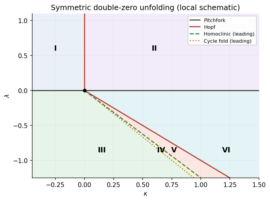
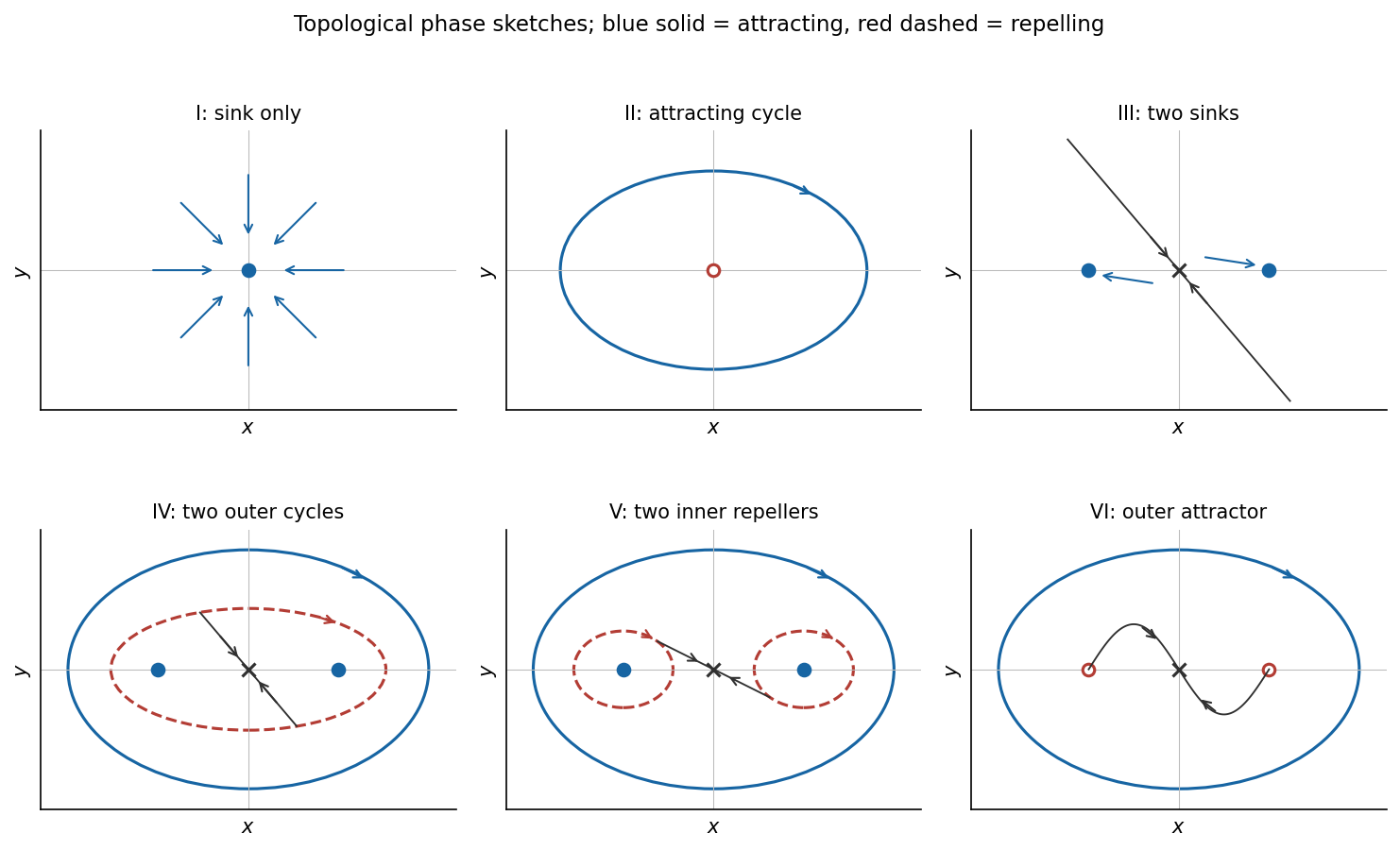
The local bifurcation curves are thereforeFor $\kappa \ne 0$ on the pitchfork curve, a leading centre-manifold equation is $\dot{x}=(\lambda x+x^3)/\kappa +\cdots$. For $\kappa <0$, with unfolding parameter $-\lambda$, the pitchfork is supercritical and creates two sink equilibria from a sink equilibrium that becomes a saddle equilibrium. For $\kappa >0$ it is subcritical in the centre direction; the nonzero branches are unstable, and the transverse eigenvalue is also positive. The origin of parameter space is a reflection-symmetric double-zero degeneration.

To determine Hopf criticality at the origin, use the energy $E=y^2/2+\lambda x^2/2+x^4/4$, whose derivative is $(\kappa -x^2)y^2$. For a small nearly harmonic oscillation $x=R\cos (\sqrt{\lambda }t)$, averaging gives $\dot{R}=\kappa R/2-R^3/8+\cdots$. Thus this Hopf bifurcation is supercritical and creates an attracting periodic orbit for $\kappa >0$. By the supplied opposite-criticality fact, the simultaneous Hopf bifurcations at the two nonzero equilibria are subcritical. A direct calculation confirms this: writing $x=\sqrt{-\lambda }+X$, $Y=-y/\sqrt{-2\lambda }$ puts the cubic radial coefficient at $1/4>0$, including the contribution from the quadratic terms.

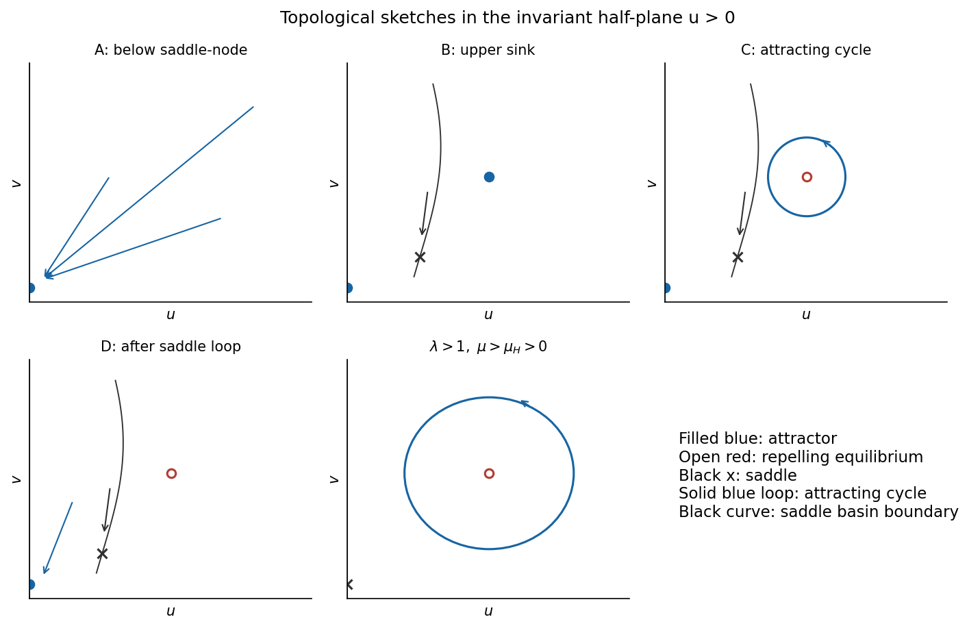
The figure includes these local curves and the global curves derived below. All lines emerging from the double-zero point are local asymptotic sketches.

With primes denoting differentiation in $\tau$, the weighted scaling givesIndeed $\dot{x}={\epsilon }^2{u}^{\prime }$ and $\dot{y}={\epsilon }^3{v}^{\prime }$, so the damping terms carry one extra power of $\epsilon$. ConsequentlyAt $\epsilon =0$ this proves conservation of $H$ directly.

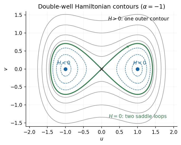
For $\alpha =-a_0^2<0$, the potential is a double well. Its minima are at $u=\pm a_0$, where $H=-a_0^4/4$; these are centre equilibria. The origin is a saddle equilibrium and has $H=0$. Energies $-a_0^4/4<H<0$ give two separate closed contours, one in each well. Energies $H>0$ give a single closed contour surrounding both wells. The intervening figure-eight consists of two homoclinic loops:Their outer turning points are $u=\pm \sqrt{2}{a}_0$. The positive loop, for example, is parametrized by $u=\sqrt{2}{a}_0\mathrm{sech}(a_0\tau )$, $v=u^{\prime }$.

A returning orbit must have zero net change of the energy. To first order, integrate the perturbation along either unperturbed homoclinic loop:For the positive loop, $v_h=\pm u_h\sqrt{a_0^2-u_h^2/2}$; the outward and inward halves contribute equally. ThereforeandThe integrals follow by substituting $w=a_0^2-u^2/2$; for the second one use $u^2=2(a_0^2-w)$. HenceThe equality in rescaled parameters is the leading Melnikov balance, not an assertion that the entire finite-parameter bifurcation curve is exactly straight. Reflection symmetry makes both saddle equilibrium loops occur together. The global curve lies below the nonzero-equilibrium Hopf line $\kappa =-\lambda$, as shown in the parameter sketch.

The relevant saddle equilibrium is the origin, with eigenvaluesFor $\lambda <0$, they have opposite signs. Its saddle index isnear the homoclinic curve, because that curve has $\kappa >0$. Along its leading asymptote, $\delta =1-\frac{4}{5}\sqrt{-\lambda }+o(\sqrt{-\lambda })$.

A local passage near the saddle equilibrium contributes a power $s^{\delta }$ to the return map. Because $\delta <1$, its derivative becomes large as the orbit approaches the separatrix. The periodic orbits meeting the loops are therefore unstable, and their periods diverge logarithmically. On the side between the homoclinic and subcritical Hopf curves there are two unstable single-well periodic orbits, surrounding the two sink equilibria. On crossing the double-loop curve downward, they join into one unstable outer periodic orbit surrounding both wells. The attracting outer periodic orbit is not the one that collides with the saddle equilibrium: it persists across this global event.

The unstable outer periodic orbit must subsequently meet that attracting outer periodic orbit in a fold of periodic orbits. This extra curve is required to obtain the six-region diagram. One can see its position from the same energy-balance calculation. After normalizing $a_0=1$, an outer Hamiltonian contour with $H>0$ selectsAt $H=0$, $B=4/5$. The derivative of the denominator diverges positively there, while that of the numerator stays finite, so $B$ initially decreases. Rescaling at large $H$ gives $B(H)\propto \sqrt{H}$, so it eventually increases. At its minimum the stable and unstable selected periodic orbits meet. Thus the outer-cycle fold in a weakly perturbed double-well oscillator has ${\kappa }_{\mathrm{fold}}=c_f(-\lambda )+o(|\lambda |)$ with $0<c_f<4/5$; quadrature gives $c_f\simeq 0.75226$. The decreasing portion of $B(H)$ selects the unstable periodic orbit, and the increasing portion selects the stable one, since the energy drift has sign $\beta -B(H)$.

Write $F={\kappa }_{\mathrm{fold}}(\lambda )$, $G={\kappa }_{\mathrm{hom}}(\lambda )$ and $H=-\lambda$ for $\lambda <0$, so $0<F<G<H$ near the double-zero point. The six open regions are:

The changes III–IV, IV–V and V–VI are respectively a fold of periodic orbits, the double homoclinic event, and the two subcritical Hopf bifurcations. Thus the unstable periodic orbits from the subcritical Hopf bifurcations, the expanding saddle equilibrium passage, and the attracting periodic orbit from the other Hopf bifurcation fit into one consistent portrait.

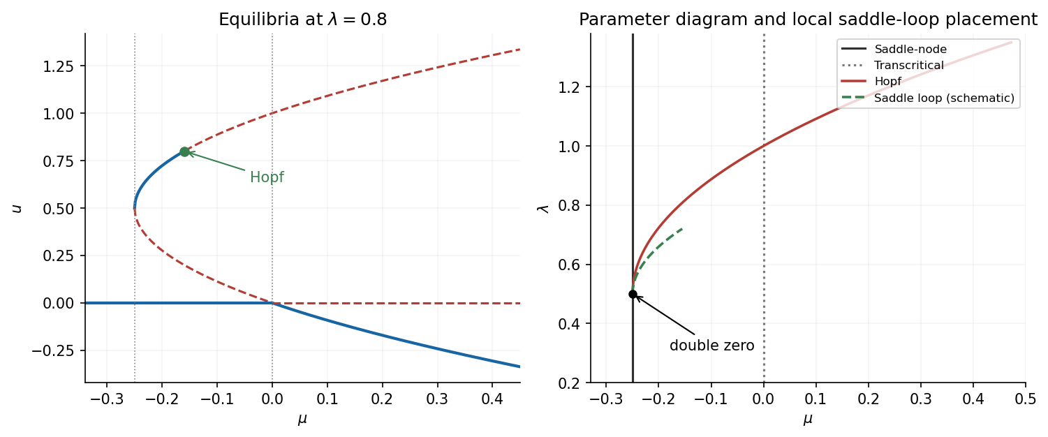
The first equation factors as $\dot{u}=u(\mu +u-v)$ and the second gives $v=u^2$ at an equilibrium. HenceThe two nonzero branches exist for $\mu \ge -1/4$, coincide at equality, and the lower branch coincides with the origin at $\mu =0$. For $-1/4<\mu <0$ both are in $u>0$; for $\mu >0$, $P_{-}$ has $u<0$ and $P_{+}$ has $u>0$.

At the origin, the eigenvalues are $\mu ,-\lambda$. At any nonzero equilibrium $(s,s^2)$, using $\mu =s^2-s$ givesThus $P_{-}$ is a saddle equilibrium for $-1/4<\mu <0$, and a sink equilibrium for $\mu >0$ when it lies in the negative half-plane. The upper branch has positive determinant and is stable for $s_{+}<\lambda$, unstable for $s_{+}>\lambda$. These statements include the existence and stability information needed for the subsequent diagrams.

At $\mu =-1/4$, the two branches meet at $(1/2,1/4)$. The eigenvalues there are $0$ and $1/2-\lambda$. For $\lambda \ne 1/2$, the nonzero quadratic term and transverse stability identify a saddle-node bifurcation. If $\lambda >1/2$, it creates a sink equilibrium and a saddle equilibrium as $\mu$ increases; if $\lambda <1/2$, it creates a source equilibrium and a saddle equilibrium. At $\lambda =1/2$, the zero eigenvalue is double and the ordinary saddle-node description needs the two-parameter unfolding.

At $\mu =0$, the origin and lower branch cross. Since $s_{-}=-\mu +O({\mu }^2)$, the branches cross transversely in the $(\mu ,u)$ diagram. The origin changes from a sink equilibrium to a saddle equilibrium as $\mu$ increases through zero; the lower branch changes from a positive-$u$ saddle equilibrium to a negative-$u$ sink equilibrium. This is a transcritical bifurcation. A local centre-manifold calculation also gives $\dot{u}=\mu u+u^2+\cdots$, because $v=O(u^2)$ and the transverse eigenvalue is $-\lambda <0$.

The figure uses a representative $\lambda >1/2$; the upper branch's additional Hopf change is indicated. For $\lambda <1/2$ the upper branch is unstable everywhere on its existence interval. The exact trace criterion in part (a) specifies stability for every fixed positive $\lambda$.

Only the upper equilibrium can have zero trace with positive determinant. Setting $s_{+}=\lambda$ givesAt this point the determinant is ${\lambda }^2(2\lambda -1)>0$, so the angular frequency is $\lambda \sqrt{2\lambda -1}$. Moreover $d{s}_{+}/d\mu =1/\sqrt{1+4\mu }>0$, so the trace crosses zero transversely as $\mu$ increases. The stipulated supercritical Hopf bifurcation creates a stable periodic orbit on the side $\mu >{\mu }_H$ where the upper equilibrium becomes unstable.

The steady-state curves are the vertical lines $\mu =-1/4$ and $\mu =0$ in the $(\mu ,\lambda )$ plane. The Hopf parabola has its endpoint atThere the Jacobian has trace and determinant zero but is not the zero matrix: it has a nilpotent Jordan block. This is the codimension-two Takens-Bogdanov point. The intersection of the Hopf curve with $\mu =0$ at $\lambda =1$ concerns a different equilibrium from the transcritical crossing at the origin; it is not another double-zero equilibrium.

The global curve is a homoclinic connection to the lower positive equilibrium, which is the saddle equilibrium created at the saddle-node bifurcation. Near $\lambda =1/2$ on the side $\lambda >1/2$, place it attangent to $\mu =-1/4$ at the double-zero point. The stable periodic orbit occupies the strip ${\mu }_H<\mu <{\mu }_G$ and approaches the saddle equilibrium on the upper boundary. The dashed curve in the two-parameter figure indicates this local placement; its drawn numerical coefficient is schematic, not a computed global-bifurcation formula.

This placement is consistent with the supplied normal form. Its centre equilibrium has a supercritical Hopf bifurcation, and its saddle equilibrium has negative trace on the relevant loop branch, allowing a stable periodic orbit to disappear in the saddle equilibrium loop. No global-curve calculation is required here.

The four nearby portrait types in $u>0$ can be organized by increasing $\mu$ at fixed $\lambda >1/2$ close to $1/2$:

The no-cycle region D continues around the double-zero point onto the $\lambda <1/2$ side. The sketches distinguish the boundary origin from the two interior equilibria and show the periodic orbit only in region C.

Here $\mu >{\mu }_H=\lambda (\lambda -1)>0$. The origin is a saddle equilibrium, $P_{+}$ is repelling, and $P_{-}$ lies in $u<0$. Thus there is no saddle equilibrium in the interior of $u>0$ to which this periodic orbit could become homoclinic. The origin cannot supply the missing loop: the line $u=0$ is invariant and is precisely its local stable manifold. An orbit in $u>0$ cannot lie on that stable manifold, so the positive periodic orbit cannot close into a homoclinic orbit to the origin either.

The outgoing trajectories do not escape to infinity in this regime. To see the large-amplitude turning mechanism, put $w=v/u$ once $v\ge 0$. Direct differentiation givesSince $\lambda >1$, the quadratic $w^2-w+\lambda$ is uniformly positive. At large $u$ while $0\le w\le 1$, $\dot{w}$ is bounded below by a positive multiple of $u$, whereas $\dot{u}/u\le \mu +u$. Thus $w$ rises by a fixed amount per bounded increase in $\log u$: the trajectory reaches $w>1$ and then $w>1+\mu /u$, where $\dot{u}<0$, before $u$ can diverge. The same estimate bounds repeated outgoing excursions; large positive $v$ also decreases when $v>u^2$. Initially negative $v$ increases until it becomes nonnegative. These nullcline and ratio estimates give bounded forward excursions.

The repelling upper equilibrium is therefore surrounded by recurrent trajectories, and the Poincaré-Bendixson alternative supplies periodic motion rather than a saddle equilibrium connection. The supercritical attracting periodic orbit persists in the displayed regime, with trajectories spiralling away from the upper equilibrium and approaching it. The last panel of the portrait figure shows this behavior; the boundary stable manifold of the origin is kept separate.

The change of time is $d\tau /dt=u$, which is positive in the half-plane under consideration. Dividing the two approximate equations by $u$ givesSet $w=v-\mu$. The inhomogeneous system becomes $(u,w{)}^{\prime }=(u-w,\lambda u)$, with eigenvalues $(1\pm \sqrt{1-4\lambda })/2$. For $\lambda >1/4$, write $\omega =\sqrt{4\lambda -1}/2$. Integrating with the prescribed initial data givesandThese expressions also verify both initial values and their initial derivatives. For fixed $\mu >0$ and small $h,v_0$ on the outgoing branch, the sine coefficient in $u$ is positive and dominates the initial cosine term. The first return to small $u$ is near the first positive zero, $\omega \tau \simeq \pi$. HenceThe factor is a half-turn of the growing spiral, not its full rotation period. After this excursion the approximate trajectory approaches the small-$u$, large-$v$ region. In the full system the term $-\lambda v$, omitted during the large excursion, allows the motion to descend along that region and return.

As $\lambda \downarrow 1/4$, the rescaled excursion time diverges and the factor $e^{\tau /2}$ produces arbitrarily large excursions. At the critical value the matrix is a nontrivial Jordan block, and the limiting formula isFor the small outgoing initial data this is positive and unbounded: the unstable manifold no longer turns back. Below $1/4$ the two eigenvalues are real and positive, so there is again no oscillatory return. This quadratic escape desingularization explains loss of the periodic orbit at infinity, together with the unstable-manifold escape, as $\lambda$ decreases through $1/4$. It is not a finite homoclinic bifurcation to the origin. The divergent $\tau$ travel time must not be identified with the physical period without integrating $dt=d\tau /u$; the time change becomes singular near $u=0$.

A global bifurcation joins two mechanisms: a long passage near a hyperbolic equilibrium point and a finite excursion returning the unstable manifold to its neighborhood. Eigenvalue ratios control the local passage, while the geometry of the global return decides reinjection, folding and trapping. In the real symmetric case there are two returning branches and a power-law cusp. In the saddle-focus case rotation adds infinitely many oscillations to that cusp. The following maps display both mechanisms explicitly.

For the Lorenz configuration, enter on $z=h$ at $(x,y,h)$ and leave on $x=sh$, where $s=\mathrm{sgn}(x)$. Solving the linear flow gives a flight timePut $\gamma =-\hat{\lambda }/{\lambda }_{+}>\delta =-{\lambda }_{-}/{\lambda }_{+}$. The outgoing coordinates areThe smooth global map from each outgoing section to the incoming section has, to leading order,up to the choice of which unstable branch carries the sign of $\nu$. Reflection symmetry makes the offsets opposite and the leading coefficients equal. Since the stable transverse coordinate is multiplied by the higher power $|x{|}^{\gamma }$, it contributes only subleading terms to the leading scalar map. Absorbing powers of $h$ into a positive constant gives the Lorenz power return mapThe line $x=0$ lies on the stable manifold and has no finite return; the discontinuity is therefore a genuine missing return, not an arbitrary value to assign at zero.

If $\delta >1$, the derivative $A\delta |x{|}^{\delta -1}$ tends to zero. For $\mu <0$, there are two attracting fixed points, $x=\pm s$ with $s=-\mu +A{s}^{\delta }\simeq -\mu$. They describe two symmetry-related one-lobe attracting flow periodic orbits. For $\mu >0$, the orbit alternates between $s$ and $-s$, where $s=\mu -A{s}^{\delta }\simeq \mu$; its multiplier is $(A\delta s^{\delta -1}{)}^2<1$. This represents one attracting flow periodic orbit traversing both lobes. At $\mu =0$ the two homoclinic loops meet: this is the contracting gluing scenario, with diverging flow period at the connection.

If $\delta <1$, the local derivative is unbounded, and the small periodic orbits are repelling in the expanding return direction. For $\mu >0$, the small positive fixed point has $s\simeq (\mu /A{)}^{1/\delta }$, with a multiplier tending to infinity; there is a symmetry-related negative fixed point as well. More complex motion follows from the two branches, not merely from a large derivative at one fixed point. Choose $I=[-c\mu ,c\mu ]$ with $0<c<1$. The inverse branches areFor sufficiently small positive $\mu$, both lie inside $I$, their images are disjoint, and their derivatives are $O({\mu }^{1/\delta -1})\to 0$. Nested inverse images for every infinite sign sequence therefore define a Cantor invariant set. Iterating the forward map shifts the sequence. This constructs periodic itineraries of every symbolic period and nonperiodic itineraries; transverse contraction in the full return turns the expanding two-strip mechanism into a horseshoe.

This is the local chaotic Lorenz mechanism. A robust attracting Lorenz set additionally needs a global trapping region and the appropriate return properties. The scalar asymptote and $\delta <1$ alone do not prove that every nearby orbit is attracted to one chaotic set; periodic windows, escaping orbits and other global returns must be distinguished. Symmetry is crucial to obtaining the two homoclinic branches together in a single parameter variation.

In cylindrical coordinates the saddle-focus linearization isUse a small incoming neighborhood of the stated section point $(\rho ,0,-\mu )$. A nearby incoming cylinder $r=\rho$ is smoothly equivalent to that section for this calculation. Denote the positive unstable passage coordinate by $x=z_{\mathrm{in}}>0$ and leave at $z=h$. ThenThe global map is smooth in the outgoing Cartesian coordinates $r_{\mathrm{out}}\cos {\theta }_{\mathrm{out}}$ and $r_{\mathrm{out}}\sin {\theta }_{\mathrm{out}}$. Its returned unstable coordinate therefore has the leading formCombining the two trigonometric terms, absorbing the fixed scales into the amplitude and phase, and using the evenness of cosine givesThe returned radial section coordinate is $\rho +O(x^{\delta })$, supplying the thin transverse direction of the full two-dimensional return. In particular its determinant has order $x^{2\delta -1}$; the exponent is also obtained by integrating the flow divergence ${\lambda }_{+}+2{\lambda }_{-}$ over the local flight. Thus $\delta >1/2$ is the volume-contracting range. Corrections from the returned radial deviation enter at order $x^{2\delta }$, smaller than the fixed-point term $x$ in this range. Only positive returned $x$ on the chosen branch belong to the scalar return domain.

For $\delta >1$,For small $\mu <0$, there is one small attracting fixed point $x=-\mu +O(|\mu {|}^{\delta })$, representing a stable long-period periodic orbit. It ends in the homoclinic connection at $\mu =0$; for $\mu >0$ there is no sufficiently small positive fixed point. The oscillations alone do not create expanding chaos when their derivative tends to zero.

For $1/2<\delta <1$, there is both net volume contraction and a positive saddle equilibrium value ${\lambda }_{+}+{\lambda }_{-}>0$. At the connection, fixed points satisfyThe right side tends to zero, while the phase runs through infinitely many rotations. There are therefore infinitely many positive fixed points accumulating at zero near successive cosine zeros. Their successive size ratios tend to $e^{-\pi /q}$ and their derivative magnitudes diverge. In the full return they are saddle equilibrium periodic orbits: one multiplier expands and the thin transverse direction contracts. Their flow periods grow as ${\lambda }_{+}^{-1}\log (h/x)$.

The oscillatory graph also supplies the complicated itineraries. Take a sufficiently small positive return interval. Near successive zero crossings, narrow monotone subintervals map across that interval with arbitrarily large slope. Two or more inverse branches contract into it, so repeated inverse choices give symbolic invariant sets just as in part (a); lifting the strips to the thin two-dimensional return gives horseshoes and infinitely many periodic orbits. This explains the Shilnikov chaotic mechanism rather than only naming it.

For nonzero splitting, the graph shifts vertically. Fixed-point tangencies with slope $+1$ create saddle-node bifurcations of periodic orbits; crossings of slope $-1$ give period doubling. Near an oscillatory extremum the derivative can be small, allowing stable periodic windows. Such thresholds accumulate geometrically toward the homoclinic parameter, interspersed with expanding returns. Hence the unfolding can contain complicated switching, arbitrarily long periods and chaos, rather than a single attracting periodic branch. This is log-periodic accumulation of Shilnikov cycles. The conclusion concerns invariant sets and possible attractors allowed by the return geometry; it does not assert that a homoclinic connection alone makes all nearby trajectories chaotic.

Write $\alpha =\pi /\sqrt{3}$ and $L={\alpha }^2+{\pi }^2=4{\pi }^2/3$. The primary streamfunction mode describes a single roll spanning the box, while the first magnetic mode describes the distortion of the vertical field by that roll. The second magnetic mode is independent of height and has twice the horizontal wavenumber, as generated by interaction of the first two modes. TakeThese satisfy all the stated boundary conditions: the sine factors vanish on the vertical walls, $\psi$ and its Laplacian vanish on every wall, and $A_z$ vanishes at the horizontal walls.

Let $J(f,g)=f_x{g}_z-f_z{g}_x$. Since ${\nabla }^4\psi =L^2\psi$, $J(\psi ,{\nabla }^4\psi )=0$. The magnetic Jacobians areandProjecting onto the three retained Fourier modes and discarding the generated third horizontal harmonic yields, in the original time,Here $4{\alpha }^2=L$, so the second magnetic mode has the same linear diffusion rate as the first.

Choose $\tau =Lt$ and normalize the amplitudes byFor example the coefficient of $a$ in $b^{\prime }$ is $(\pi /L)(4\sqrt{2})/(3\sqrt{2}/\pi )=1$, and that of $ab$ in $c^{\prime }$ is $3$. The linear momentum coefficients become $r=R{\alpha }^2/L^3=9R/(64{\pi }^4)$ and $q=Q{\pi }^2/L^2=9Q/(16{\pi }^2)$. ThereforeThis is three-mode porous magnetoconvection. Because the nonlinear magnetic advection generates a discarded harmonic, it is a Galerkin approximation, not an exact three-dimensional invariant subspace of the partial differential equations.

At the no-convection equilibrium $(a,b,c)=(0,0,0)$, one eigenvalue is $-\zeta$ and the other two come fromTheir trace and determinant areA zero eigenvalue occurs at $r=1+q$. If $q<\zeta /\sigma$, the other two eigenvalues are negative, and the stationary bifurcation is the pitchfork analyzed in part (c). For $q>\zeta /\sigma$ the transverse eigenvalue is positive instead.

An imaginary pair occurs at $r=1+\zeta /\sigma$, provided $q>\zeta /\sigma$, becauseThe trace crosses zero with derivative $\sigma >0$. The cubic coupling is nondegenerate here: at criticality, putting $K=\sigma \zeta q$ reduces the oscillatory variables toFor $a=R\cos ({\omega }_H\tau )$, the forced second harmonic of $c$ has sine coefficient $9R^2\zeta {\omega }_H/[2K({\zeta }^2+4{\omega }_H^2)]$. Averaging the derivative of $(a^{\prime 2}+{\omega }_H^2{a}^2)/2$ consequently gives $-9\zeta {\omega }_H^2{R}^4/[8({\zeta }^2+4{\omega }_H^2)]<0$. Thus the Hopf bifurcation is nondegenerate and supercritical.

The two thresholds meet atHere the planar block is nonzero but has trace and determinant zero, while the third eigenvalue remains negative. It is a reflection-symmetric double-zero, codimension-two point; the ordinary simple-eigenvalue reduction of part (c) is not valid there.

Fix $\mu =r-1-q$ and $0<q<\zeta /\sigma$. The noncritical eigenvalues at $\mu =0$ are $-\zeta$ and $\sigma q-\zeta <0$. Include the constant parameter as an additional centre variable. Symmetry permits expansionswhere the omitted terms in the reduced equation have order ${\mu }^{2}a,\mu a^3,a^5$. At $\mu =0$, $a^{\prime }$ begins at cubic order, so $c^{\prime }=c_a{a}^{\prime }$ begins at fourth order. The $c$ equation therefore gives $c_2=3/{\zeta }^2$.

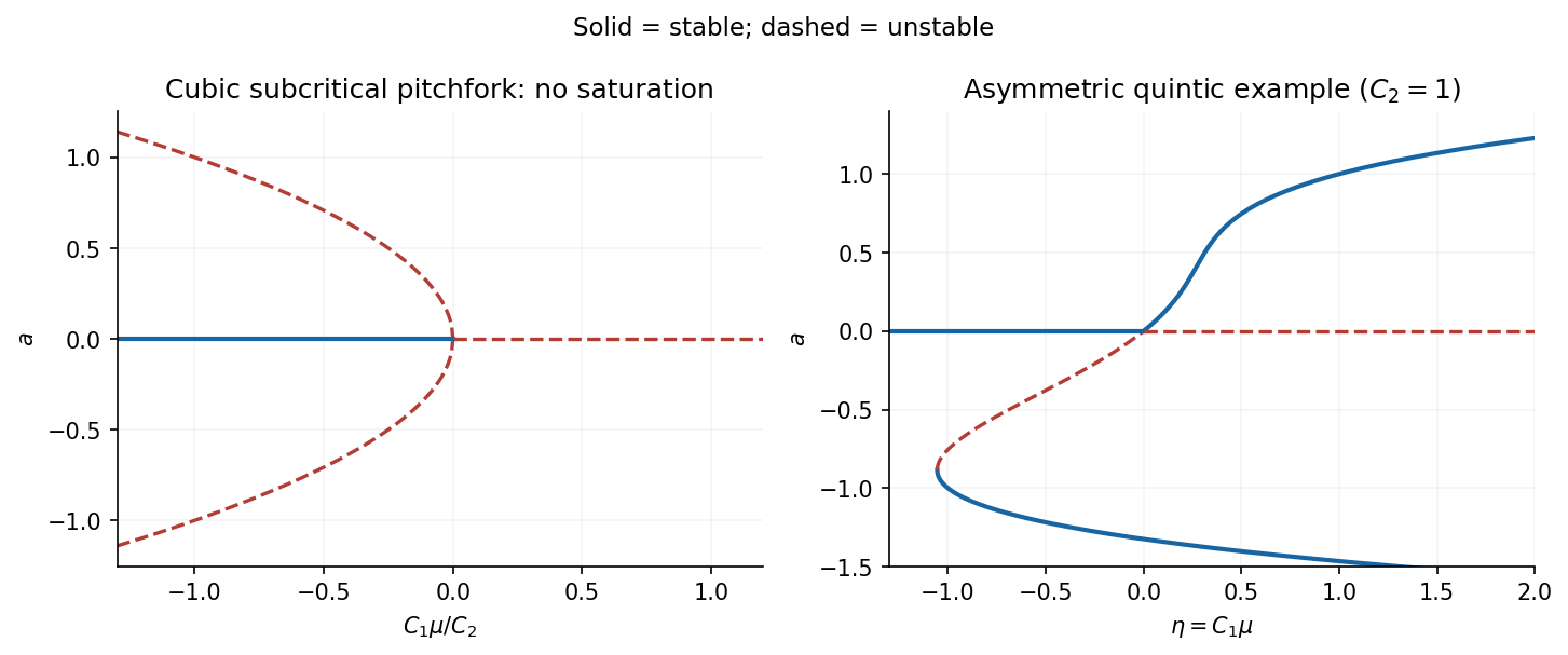
The invariance equation for $b$ must retain $b_a{a}^{\prime }=a^{\prime }/\zeta +\cdots$. From the first equation,Equating coefficients in $b_a{a}^{\prime }=a-\zeta b-ac$ givesHenceand the required reduced equation isBoth coefficients are positive. Thus the bifurcation is a subcritical pitchfork: the no-convection state is stable for $\mu <0$ and unstable for $\mu >0$. The small nonzero branches lie on the stable-origin side,and are unstable, since the derivative of the reduced vector field there is $-2C_1\mu >0$. Their two transverse directions remain stable, making them saddle equilibrium equilibria in the three-dimensional model. Setting $b^{\prime }=c^{\prime }=0$ without the invariance correction would incorrectly omit the common factor $(1-\sigma q/\zeta {)}^{-1}$. This is the cubic centre-manifold reduction of porous magnetoconvection.

For $\mu >0$, the cubic equation has the same sign as $a$ everywhere away from zero: small positive or negative disturbances grow without saturation, and the cubic truncation even predicts finite-time blow-up. An amplitude of convection cannot grow indefinitely under that local approximation. The conclusion is that additional nonlinear physics and higher-order terms are needed, not that the small-amplitude reduction is valid at arbitrarily large amplitude.

For the modified equation put $\eta =C_1\mu$ and $C=C_2>0$. It can be writtenThe quintic term points inward for sufficiently large $|a|$, so all forward solutions are bounded and approach equilibria in this scalar problem. The quadratic term breaks $a\mapsto -a$ symmetry. Besides $a=0$, the equilibrium diagram isThis stability criterion follows from $f^{\prime }(a)=-a{g}^{\prime }(a)$ on the equilibrium curve, where $g^{\prime }=1-2Ca+4a^3$. Near zero the new branch is $a=\eta +O({\eta }^2)$, crossing the trivial branch transcritically. It is unstable for small negative $\eta$ and stable for small positive $\eta$; the trivial branch has the opposite stability.

The negative-amplitude part of $g$ has exactly one minimum. Above its negative fold value but below zero, a stable finite-amplitude negative state coexists with the stable origin, separated by an unstable negative equilibrium. This gives hysteresis and finite-amplitude triggering of convection. For positive $\eta$ the origin is unstable and stable nonzero states provide saturation. Additional positive-amplitude folds depend on $C$: $g^{\prime }$ has two positive roots for $C>3/2$, a double root at $C=3/2$ and none for $C<3/2$, so further multistability can occur. The right-hand figure illustrates $C=1$, without those extra positive folds; it does not assume that every possible $C_2$ gives that same detailed diagram. These are the qualitative changes in quintic saturation of a symmetry-broken pitchfork.