Put , the seismic impedance. In a uniform medium, define and . The field equations giveThus and , with arbitrary independent profiles . Reconstruction givesThe two characteristic components therefore have , and , .
The kinetic plus elastic energy mass density is . Multiplying the equations by and yields . Hence the elastic-wave energy flux is . For a pure forward wave ; for a pure backward wave . In the mixture the cross terms cancel, giving . Strict sign holds for nonzero components.
Let the positive real material parameters depend on but not on time. Define the flux-normalized elastic characteristic amplitudes and logarithmic seismic impedance gradientWrite and . Then , , and direct substitution givesFor example, the first relation uses and ; the second uses . Adding and subtracting now provesThe original PDF has these two first-order equations. The TeX mistakenly combines them into ratios, which must not be used. A seismic impedance gradient couples forward and backward wave amplitudes even when the local wave speed is allowed to vary.
Use a time-harmonic wave with time dependence and let the same symbols denote phasors. The wave amplitude vector obeysAt fixed material contrast, the stated low-frequency condition permits neglecting the diagonal frequency term to zeroth order. All remaining coefficient matrices are scalar multiples of the same exchange matrix, so they commute. Withthe transfer relation isSolve the second row for the outgoing left wave amplitude and substitute in the first. Since , this gives the zero-frequency scattering through an elastic layer coefficientsThus the zero-frequency limit depends only on the endpoint seismic impedances. Monotonicity supports the given scale comparison but is not needed to integrate the zero-frequency equation. If in a monotone profile, seismic impedance is constant: there is no directional coupling, with only wave phase accumulation at nonzero frequency.
At a sharp interface, continuity of velocity and traction gives, for unit incident velocity from the left,Thus and . Normalizing the transmitted velocity by its elastic-wave energy flux gives , exactly the result above. Right incidence gives the reversed reflection sign and the same flux-normalized transmission. A stress reflection coefficient has the opposite sign to the velocity reflection coefficient; the convention matters.
Put and . The incoming-to-outgoing matrix is , with . Therefore , proving equality of incoming and outgoing time-averaged flux for arbitrary coherent incident wave amplitudes, not just incidence from one side.
For all real frequencies the harmonic equations instead giveTheir right sides are equal; the diagonal terms have zero real contribution. ConsequentlyThe mean flux for real-part phasors is . Evaluating it at the two endpoints proves exactly that total outgoing flux equals total incoming flux at every real frequency. This relies on real lossless moduli and mass density; absorption would change the identity.
Take a stable isotropic elastic material with mass density and Lamé parameters , where and . Its elastic stiffness tensor isThe P wave is longitudinal and the S wave transverse. The wavefront-transport alternative and all three steps of the Love wave alternative are given below.
Assume the coefficients are sufficiently differentiable in the region considered, with no material discontinuity or caustic at the front. Let describe arrival time, the slowness vector, and the unit elastic wave propagation normal. For any field, its jump is the value immediately behind the front minus that immediately ahead. If the first nonzero jump occurs in the kth time derivative, , writeA smooth background may be added without changing these leading jumps. Since , differentiation expresses spatial jumps in terms of and time-derivative jumps. The restriction lets displacement field and its first time derivative remain continuous and avoids an imposed impulsive source at the front.
Insert this local expansion in . The coefficient of isFor isotropic elasticity the slowness acoustic matrix is . Its longitudinal eigenvalue is . The P branch therefore gives the eikonal equation and polarizationThe next coefficient, , isThe matrix on the left is symmetric and annihilates . Project onto to obtain its solvability condition. Put . The two projected terms can be evaluated without dropping gradients of mass density or moduli:These identities use , hence , and . Their curvature terms cancel, leavingMultiplying by proves the requested P-wavefront discontinuity transport law,The wave amplitude here is real for a real jump; a complex wave amplitude uses the corresponding modulus-squared law. An elastic ray follows , with arclength and . If is the infinitesimal cross-sectional area of a neighboring ray tube, . Thus is constant along that tube, the ray-tube conservation for a P-wave jump. This defines the geometrical spreading and shows why the wave amplitude changes with material properties even before attenuation is considered. At a caustic the simple ray-tube wave amplitude is singular and a uniform local description is needed.
Choose depth positive downwards, the free surface at and the interface at . A Love wave has only transverse displacement field . Take , , and defineA trapped mode requires , so both are positive. The SH equations are in the layer and in the half-space. Zero shear traction at the free surface and decay at large depth selectContinuity of displacement field and shear traction at gives and . ConsequentlySubstituting the definitions of yields the requested speed-frequency dispersion relation. For negative frequency use in both vertical wavenumbers; the real displacement field has conjugate frequency partners. Neither equality in the trapped-speed interval gives a strictly localized finite-frequency Love mode.
Refer all layer wave amplitudes to the lower interface. Let a downward incident SH displacement field have unit wave amplitude there, an upward reflected wave have wave amplitude , and the decaying half-space wave wave amplitude . Interface continuity givesSolving these equations proves the Love-wave interface reflection phase and transmission wave amplitude:Thus : the evanescent substrate field has nonzero wave amplitude but no net downward mean flux. At the traction-free top, an upward incident wave and its downward reflection must have canceling derivatives, so their displacement field reflection coefficient is .
A layer wave acquires wave phase during a complete round trip. Constructive interference requiresTaking the tangent gives again . The reflection phases, rather than only geometric travel distance, are essential to the mode condition.
At , the half-space decay exponent tends to zero and the dispersion relation requires . These are the Love-wave cutoff frequencies,An overtone exists strictly above its cutoff. At the cutoff its half-space field is constant in depth rather than decaying, so it is a limiting nonlocalized state, not a trapped finite-energy eigenfunction. The fundamental has cutoff zero and exists for every positive frequency. Each fixed branch approaches from above at high frequency. The half-space penetration depth diverges on approach to cutoff.
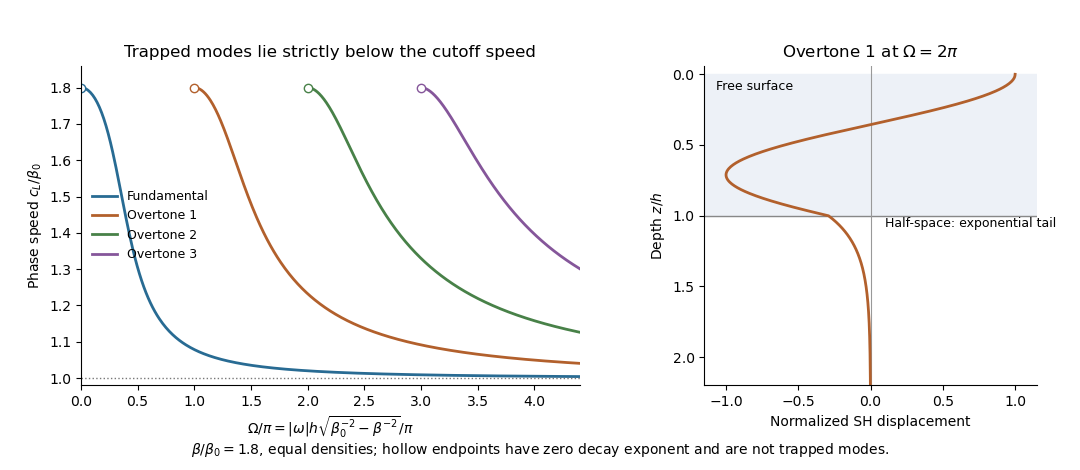
Love-wave dispersion branches above their cutoffs and an overtone displacement profile across the layer interface
. Details. 
Use the same real elastic stiffness tensor for both fields, including its minor and major symmetries, and let , with outward unit boundary normal . No complex conjugation is needed for the initial bilinear identity. DefineThe divergence has two force-balance terms and two cross-gradient terms. The latter cancel becausethis follows by exchanging the two strain-gradient factors using major symmetry and the minor pair symmetries. The frequency-domain equations then giveIntegrating and applying the divergence theorem provesThis is the Betti identity for elastodynamic fields. Spatially varying stiffness is allowed because its derivatives remain inside the divergence. The original PDF's constitutive contraction is ; the TeX's repeated displacement field index is erroneous.
In the bilinear identity choose field to be the complex conjugate of the field at frequency , equivalently its partner, and field to be the field itself. The squared frequencies are equal, so the mass density terms cancel:Multiply by and use , to obtainFor the real fields defined in this question as the sum of positive and negative frequency components, time averaging cancels the terms. Their mean body-force work mass density is exactly , and their outward mean elastic-wave energy flux is . Thus mean body-force power equals mean outward boundary power. Mean stored energy does not accumulate in a periodic steady field.
There is no extra factor here: the specified real field is , not . For the latter phasor convention, both averages instead have the usual factor . At velocity and both powers vanish.
Choose field to be at frequency , and field to be at . Zero body forces and zero boundary tractions make all source and surface terms vanish. ThereforeFor distinct squared frequencies this proves weighted orthogonality,Assume positive mass density bounded above and below and finite-energy fields in the ordinary bounded domain. The weighted space is a separable Hilbert space. Select one unit eigenfunction for each distinct squared frequency. They form an orthonormal set. Let be a countable dense subset of ; assign to each eigenfunction a point within distance . Two orthogonal unit eigenfunctions have distance , so the same cannot be assigned to both. This gives an injection into a countable set.
Hence there are at most countably many squared eigenfrequencies, and at most twice that many signed frequencies. Multiplicity at one frequency does not change the argument. A zero frequency associated with rigid translations or rotations is included. This proves the countability of elastic eigenfrequencies directly; proving discreteness or finite multiplicity would require additional spectral regularity arguments.
If two harmonic solutions have the same body force and prescribed boundary traction, their difference has no body force and is traction-free. A nonzero difference would therefore be a free eigenfunction at that frequency. For any frequency outside the countable exceptional set found above, the difference must vanish, so the forced boundary-value solution, when it exists, is unique. At an eigenfrequency, a free eigenfunction can be added to any existing solution, and a resonant forcing may fail to admit a steady harmonic response. This distinguishes uniqueness from existence.
For the full time-dependent problem, let be the difference between two fields with identical forces, tractions and initial displacement field and velocity. It obeys , zero boundary traction, and zero initial data. Its energy uniqueness for traction-driven elasticity follows by direct integration:Multiply the equation by and integrate by parts. Major symmetry turns the strain term into the derivative of elastic energy, giving . Stable elasticity makes , and gives . Thus equals its initial value zero. Even rigid zero-strain motions cannot survive these initial conditions.
The PDF correctly specifies zero initial displacement field and zero initial velocity; the TeX duplicates displacement field in the second condition. The complete causal displacement field is unique, including when its Fourier representation contains resonant modal contributions fixed by the initial data.
Use the displacement-potential convention , and harmonic dependence . Choosing the opposite sign for the shear potential changes its column sign but not the P-SV directional impedance matrix. Write , , , and . At a common point the forward potential wave amplitudes giveThe traction formulas follow from and , using and . The velocity matrix has determinant , so elimination gives the P-SV directional impedance matrixIts off-diagonal entries are real and antisymmetric. ThereforeWith real-part phasors, the outward flux is , sofor every nonzero forward displacement field. Mass density and angular frequency are essential to this flux coefficient; both appear correctly in the PDF.
For downward-phase reversal, the P-SV displacement potentials instead produceEliminating the potentials as before givesThe Hermitian part is negative definite, and consequentlyfor a nonzero backward displacement field. The P potential must use vertical wavenumber and the S potential , as in the original PDF; the TeX incorrectly gives the shear wavenumber for both.
Define . Its antisymmetric off-diagonal entries cancel, leavingFrom and , solve explicitly for the P-SV characteristic reconstruction:The prescribed strictly positive make this decomposition unique; a grazing or evanescent branch is outside these assumptions.
In the mean flux, the two mixed directional terms arebecause makes the second scalar minus the complex conjugate of the first. The remaining self terms giveFinally use either directional velocity-potential matrix. Its weighted quadratic form satisfiesIndeed the two P-SV cross terms have coefficients and for the forward field, with the signs reversed for the backward field, so they cancel. Substitution provesThus net normal elastic-wave energy flux is the difference of the independently flux-weighted P and SV directional powers, even for coherent mixtures.
Articles by others on the same topic
There are currently no matching articles.