Past exam of the mathematics course of the University of Cambridge / 2006 / iii / Paper 49 (Advanced Quantum Field Theory)

Work in units $\hslash =1$ and with the particle mass absorbed into the stated kinetic term. Divide the interval into $N$ pieces of length $\Delta =T/N$. For a suitable self-adjoint Hamiltonian operator, the Trotter product formula gives the regulated limitInsert $1=\int d{q}_j|q_j⟩⟨q_j|$ between neighboring factors. Because $V(\hat{q})$ is diagonal in the position operator basis, the given free-particle propagator yieldsThe exponent is the time-sliced action. Its continuum notation isThe measure is defined by the displayed finite-dimensional limits and their normalization, not by a translation-invariant flat measure on an infinite-dimensional space. The oscillatory limit needs a damping/analytic-continuation prescription. This is the time-sliced configuration-space path integral derived from the operator kernel.

For a quadratic potential energy, write $q=q_c+\eta$, where the classical path satisfies ${\ddot{q}}_c+V^{\prime }(q_c)=0$ and the endpoint conditions, and $\eta (0)=\eta (T)=0$. Expansion is exact:Integration by parts makes the linear term equal to $-[{\int }_0^T({\ddot{q}}_c+V^{\prime }(q_c))\eta dt]$, since the endpoint term vanishes. It is zero by the Euler-Lagrange equation. Also $V^{\prime \prime }$ is constant, independent of the endpoints. Thus classical-path factorization of a quadratic path integral is exact:Only the classical action carries the endpoint dependence.

Let $D={\partial }_t^2+V^{\prime \prime }$ on homogeneous Dirichlet boundary conditions. Expand $\eta$ in its normalized eigenfunctions, with eigenvalues ${\lambda }_n$. The fluctuation integral becomes a product of regulated integrals $\int d{a}_n\exp (-i{\lambda }_n{a}_n^2/2)$. Each is proportional to ${\lambda }_n^{-1/2}$, with a prescribed complex phase. Relative to $D_0={\partial }_t^2$, the normalization is thereforeThe subscript denotes the Dirichlet operator domain, and the square-root branch is continued from the free kernel with its convergence prescription. Equivalently one can use determinants of $-D$ and $-D_0$. For $V^{\prime \prime }={\omega }^2$, the Dirichlet oscillator determinant ratio isThis also checks the free limit. At conjugate times, the fluctuation operator has a zero eigenvalue and the ordinary finite-prefactor expression fails; the kernel is obtained by distributional continuation. Away from these times the classical boundary problem is unique and the stated factorization applies directly.

For the infinite-time oscillator with an external source, use vacuum boundary conditions and the Feynman i-epsilon prescription. For a smooth source of compact support, defineThe imaginary term damps the real-field integral. Integration by parts gives $S_{ϵ}[q]=\frac{1}{2}q{A}_{ϵ}q+Jq$, with the pairings understood as time integrals. Completing the square givesTranslate the integration variable. The source-independent Gaussian functional integral is $N$, soOn Fourier modes $e^{i\omega t}$, $A_{ϵ}$ has eigenvalue ${\omega }^2-m^2+iϵ$, henceFor $m>0$, closing the contour above for $t>0$ and below for $t<0$ gives $G(t)=-i{e}^{-im|t|}/(2m)$. The physical time-ordered oscillator quantum field theory propagator is $iG$, not $G$ itself. The shifted stationary path is $q_c=-GJ$ and obeys ${\ddot{q}}_c+m^2{q}_c=J$ with the same vacuum prescription. A retarded inverse would define a different boundary problem. Dividing by the zero-source integral removes $N$ and gives the vacuum source functional of a quantum oscillator. At zero mass an additional infrared prescription is needed for the inverse on constant modes.

Use the mostly-plus Minkowski metric, so $p^2=-p_0^2+{\mathbf{p}}^2$, and the source term $+\int J\varphi$. Define the vacuum-normalized generating functional, connected generating functional, and quantum effective action byThe Legendre transform is taken after expressing $J$ in terms of $\phi$, locally where this relation is invertible. Varying it gives $\delta \Gamma /\delta \phi =J$ and ${\Gamma }^{(2)}=(W^{(2)}{)}^{-1}$. The logarithm generates connected graphs; the Legendre transform removes graphs joined by a single propagator, leaving one-particle-irreducible vertices. This sign convention is important: its classical limit is $\Gamma =-S$, consistent with the positive vertices in this question.

For the free real scalar field, integration by parts puts the action into the form $S=-\frac{1}{2}\varphi A\varphi$, where $A=-\square +m^2$ has Fourier symbol $p^2+m^2$. Include the Feynman i-epsilon prescription $A\mapsto A-i0$. Completing the square yieldsand consequentlyThe physical scalar propagator is $-i{A}^{-1}$, whereas the inverse quadratic kernel appearing in $W_0$ is $A^{-1}$. Differentiating this quadratic functional and Fourier transforming givesThe infinitesimal prescription specifies propagators and is dropped when quoting the local vertex kernel.

At the order represented by tree-level Feynman diagrams, stationary phase gives $W_{mtree}=S[\phi ]+\int J\phi$, with the classical field equation $\delta S/\delta \phi +J=0$. The Legendre transform cancels the source term, soThusOther connected tree graphs with several quartic vertices are one-particle reducible and belong to $W$, not to the proper vertices of $\Gamma$. This explains why no extra tree correction is hidden in these formulas.

The one-loop proper two-point graph is the tadpole diagram. The one-loop proper four-point graphs are the three bubble diagrams, with pairings $(12|34)$, $(13|24)$ and $(14|23)$ of the external legs. Each has Feynman-diagram symmetry factor $1/2$. The figure shows the topologies and every four-point channel; external momenta are incoming.

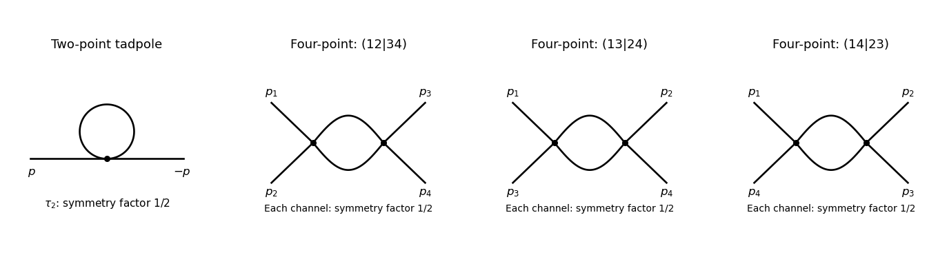
The tadpole factor can also be counted directly: there are $4\cdot 3=12$ assignments of two labeled external legs to one quartic vertex, while its $4!$ normalization leaves $12/24=1/2$. For a fixed four-point partition, the interchange of the two internal lines gives the same factor $1/2$; there are three distinct partitions. Graphs with an external self-energy insertion are one-particle reducible and are not additional contributions to ${\tau }_4$.

For the two-point divergence, perform a Wick rotation. The Euclidean tadpole contribution to the proper inverse kernel isAssume $m^2>0$ to separate the ultraviolet calculation from infrared issues. A Schwinger parameterization gives $1/(k_E^2+m^2)={\int }_0^{\infty }ds{e}^{-s(k_E^2+m^2)}$. Using the supplied Gaussian integral, initially in the convergence region, givesThe last expression provides the meromorphic dimensional regularization continuation. Set $d=4-ϵ$. Since $\Gamma (-1+ϵ/2)=-2/ϵ+O(1)$,If the coupling is written as ${\mu }^{ϵ}\lambda$, that factor multiplies the intermediate integral but does not change the displayed pole residue. The negative pole is a property of analytic continuation; it must not be inferred from the positive cutoff integrand without carrying out the continuation.

The added mass counterterm contributes $+B$ to ${\tau }_2$, because ${\Gamma }_{mtree}=-S$ and its Lagrangian term is $-B{\varphi }^2/2$. Hence cancellation requiresup to an arbitrary finite subtraction specifying the renormalization scheme. No external momentum occurs in the tadpole, so no one-loop wave-function renormalization is needed. At $m=0$ the unregulated tadpole is scaleless and vanishes in dimensional regularization; the massive calculation identifies the mass-dependent ultraviolet pole without conflating it with a massless infrared limit.

For completeness, the signs of the four-point graphs in this effective-action convention can be read from the Euclidean one-loop functional $\frac{1}{2}\mathrm{Tr}\log (A_E+\lambda {\phi }^2/2)$. Its expansion has terms $\lambda \mathrm{Tr}(A_E^{-1}{\phi }^2)/4$ and $-{\lambda }^2\mathrm{Tr}(A_E^{-1}{\phi }^2{A}_E^{-1}{\phi }^2)/16$. Differentiating four times givesThis is the Euclidean form, analytically continued to the physical external momenta. It confirms the three channel diagrams and their symmetry factors; evaluating its divergence is not needed for the requested mass counterterm.

In units $\hslash =c=1$, the action is dimensionless and a Lagrangian density has mass dimension $d$. The kinetic term therefore gives $2+2[\varphi ]=d$. Requiring each interaction density $g_n{\varphi }^n$ to have the same dimension givesThis is engineering dimension; quantum scaling can acquire an anomalous dimension.

For a connected Feynman diagram with no derivative interactions, each independent loop integration contributes $d$ powers of momentum, and each internal scalar propagator contributes $-2$. Thus its superficial degree of divergence is $D=dL-2I$. Let $V={\sum }_n{V}_n$. A connected graph has $L=I-V+1$ independent cycles, and counting the half-edges incident on vertices gives $2I+E={\sum }_{n}n{V}_n$. Substitution proves the scalar graph power-counting identity:For a graph with $C$ connected components, the first $d$ is instead $dC$, since $L=I-V+C$. The printed expression therefore uses the usual connected-graph convention. This is the overall degree under simultaneous rescaling of all loop momenta. Subgraphs can still have ultraviolet divergences when the whole graph has $D<0$, so their counterterms must be subtracted before declaring an integral finite.

When all retained couplings have nonnegative dimension, only finitely many external-leg/derivative structures can have nonnegative degree. Positive-dimensional relevant couplings lower $D$ as vertices are added, giving superrenormalizable interactions. Zero-dimensional marginal couplings give power-counting renormalizable interactions. Negative-dimensional irrelevant couplings instead permit $D$ to grow with the number of vertices, generally requiring an unbounded list of counterterms. Such nonrenormalizable interactions can still define an effective field theory to any fixed order in a low-energy expansion.

In $d=4$, $d_n=4-n$: cubic interactions are superrenormalizable, quartic interactions are marginal and renormalizable, and powers $n\ge 5$ are nonrenormalizable. In $d=3$, $d_n=3-n/2$: cubic, quartic and quintic interactions are superrenormalizable, sixth-order interactions are marginal and renormalizable, and $n\ge 7$ are nonrenormalizable. This is a power-counting classification, not a guarantee that an odd highest-power potential is bounded below. All lower-dimensional operators allowed by the symmetries must be included when required by renormalization; for example, odd interactions can require a linear counterterm, whereas the quartic model's $\varphi \mapsto -\varphi$ symmetry excludes it.

Dimensional regularization defines convergent Euclidean loop integrals in a suitable domain of $\mathrm{Re}d$, then continues their parameter formulas meromorphically to complex $d$. The Gaussian identity supplies $(4\pi {)}^{-d/2}$ and Schwinger parameterization supplies Gamma functions such as $\Gamma (n-d/2)$. Their poles encode the ultraviolet singularities near physical dimension. Noninteger complex $d$ is an analytic regulator of amplitudes, not a literal space with a noninteger number of coordinates. Masses or nonexceptional external momenta distinguish ultraviolet poles from infrared poles; scaleless integrals vanish in this convention and can hide that distinction.

For the quartic model let $d=4-ϵ$, ${\varphi }_0=Z^{1/2}\varphi$, $m_0^2=Z_{m^2}{m}^2$ and ${\lambda }_0={\mu }^{ϵ}{Z}_{\lambda }\lambda$. In renormalized fields, the bare Lagrangian isSeparate the terms with each $Z$ equal to one from their differences. The differences are field, mass and quartic counterterms. After subtracting divergent subgraphs, the remaining ultraviolet pole of a proper graph is a local polynomial in its external momenta. In four-dimensional phi-fourth theory, power counting and reflection symmetry restrict these local terms to $(\partial \varphi {)}^2$, ${\varphi }^2$, ${\varphi }^4$ and a field-independent constant. Choosing the Laurent coefficients of the three renormalization factors recursively cancels these poles at every perturbative order. The constant vacuum term is removed by the zero-source normalization. This is an order-by-order finite renormalized expansion, not a claim of convergence of the perturbation series.

The source renormalization of a scalar generating functional follows directly from rewriting the source coupling in bare variables:A general source attached to a single elementary field needs this field renormalization; its connected correlations are the ordinary renormalized Green functions. Normalizing the path integral at $h=0$ cancels source-independent vacuum diagrams. Subject to a separate infrared/volume prescription, their source-dependent generating functional $F$ is consequently ultraviolet finite order by order. For a constant source, this statement is interpreted as a formal connected expansion or a vacuum density, not as an automatically finite total logarithm in infinite spacetime.

Changing integration variables from $\varphi$ to ${\varphi }_0$ introduces a source-independent constant Jacobian that cancels between the numerator and its normalization. The resulting normalized integral depends only on ${\lambda }_0,m_0^2,h_0$ and fixed physical boundary/volume data. ThusDefine all scale derivatives at these fixed bare quantities:In a mass-independent subtraction scheme, logarithmic differentiation of the bare relations givesThe factors contain regulator poles, but the combinations determining the physical renormalization group functions have finite limits. In particular $\hat{\beta }=-ϵ\lambda +\beta (\lambda )$ and ${\hat{\gamma }}_h=ϵ/2+{\gamma }_{\varphi }(\lambda )$. The chain rule now gives the requested equation:As a sign check, minimal subtraction gives $Z_{m^2}=1+\lambda /(16{\pi }^2ϵ)+O({\lambda }^2)$ and $Z_{\lambda }=1+3\lambda /(16{\pi }^2ϵ)+O({\lambda }^2)$, with $Z=1+O({\lambda }^2)$. Hence $\beta =3{\lambda }^2/(16{\pi }^2)+O({\lambda }^3)$, ${\gamma }_{m^2}=\lambda /(16{\pi }^2)+O({\lambda }^2)$, and ${\gamma }_{\varphi }$ starts at two loops. The positive signs agree with the tadpole subtraction and the three four-point channels.

The dimensional rewriting needs care. The chosen source normalization gives $[h]=3$, $[m^2]=2$, and $[\lambda ]=0$, so $m^2/{\mu }^2$ and $h/{\mu }^3$ are the natural dimensionless parameters. For the full source functional, spacetime arguments must also be rescaled: with $y=\mu x$, write $\varphi (x)={\mu }^{(d-2)/2}\psi (y)$ and $\tilde{h}(y)={\mu }^{-3}h(y/\mu )$. The dimensionless functional then depends on $\lambda ,m^2/{\mu }^2$, the rescaled source profile, and the rescaled integration domain.

For a literal uniform source in a fixed physical spacetime volume ${\mathcal{V}}_d$, the uniform-source vacuum functional and spacetime volume relation is insteadFor example, even at $\lambda =0$ and $m^2>0$, completing the square for the constant mode givesThus the printed three-argument rewriting of the total $F$ suppresses necessary volume/source-profile data. It is valid as a dimensional shorthand only with those data understood; a dimensionless density has the three arguments, while its scale equation includes its engineering dimension. At infinite volume, the total constant-source logarithm is generally extensive and infinite even after ultraviolet renormalization.

The massless renormalization-group characteristics with a source solve the requested flow directly, independently of this notational issue. Since the mass flow is proportional to $m^2$, its zero value remains zero. Starting at a reference scale ${\mu }_{\ast }$, solveThenwith any physical volume or source-shape data retained. Where $\hat{\beta }\ne 0$, the running quantities are determined byThese equations transport matching data at one scale to any other scale on the same flow trajectory. At a zero of the beta function use the differential equations themselves, rather than divide by zero.

For the uniform-source density, set $y=h/{\mu }^3$ and $m^2=0$. At $d=4$ the corrected dimensionless equation and its local characteristic solution areThe arbitrary function $\Psi$ is fixed by boundary/matching data. If the volume is retained as a dimensionless argument $v={\mu }^4{\mathcal{V}}_4$, the full dimensionless functional obeys the same transport operator with $4v{\partial }_v$ in place of the additive $4$ term; extensivity makes the two statements equivalent. Massless zero-momentum source expansions can also have infrared singularities, so this RG solution is formal until an infrared prescription or a suitable background expansion is chosen.

An ultraviolet fixed point is a zero of the beta functions approached by the dimensionless couplings as $\mu \to \infty$. Near a single-coupling fixed point ${\lambda }_{\ast }$, perturbations obey $\delta \lambda \propto {\mu }^{{\beta }^{\prime }({\lambda }_{\ast })}$, so ${\beta }^{\prime }<0$ gives attraction in that direction. In four-dimensional quartic scalar theory, the positive one-loop beta function makes positive small coupling grow toward the ultraviolet: $1/\lambda (\mu )=1/\lambda ({\mu }_{\ast })-[3/(16{\pi }^2)]\log (\mu /{\mu }_{\ast })$. This exhibits a perturbative Landau pole, not an interacting ultraviolet fixed point. A perturbative result does not exclude hypothetical strong-coupling behavior beyond its regime.

The gauge-invariant Yang-Mills action integrates over physically equivalent configurations along each gauge orbit. At the quadratic level its gauge-field kernel has longitudinal zero directions: in momentum space $K_{\mu \nu }(k)=-k^2{\eta }_{\mu \nu }+k_{\mu }{k}_{\nu }$ satisfies $K_{\mu \nu }{k}^{\nu }=0$. It therefore has no inverse from which to construct a gauge-boson propagator. Gauge fixing both removes the redundant orbit integration and supplies an invertible quadratic operator away from the ordinary physical propagator poles.

For the covariant condition ${\partial }^{\mu }{A}_{\mu }=0$, the Faddeev-Popov determinant is that of ${\partial }^{\mu }{D}_{\mu }$. Its representation by odd Faddeev-Popov ghost fields and antighost fields produces the displayed ghost term. In a nonabelian theory $D_{\mu }$ depends on the gauge field, so the determinant is not an irrelevant constant: ghost interactions must be retained. The even Nakanishi-Lautrup field $b$ writes gauge fixing in a form with off-shell BRS symmetry. For $\xi \ne 0$, its algebraic equation is $b=-\partial \cdot A/\xi$, giving $-(\partial \cdot A{)}^2/(2\xi )$ after elimination. At $\xi =0$ it imposes the gauge condition as a Lagrange multiplier.

For the nilpotence proof, write the adjoint bracket as $[X,Y{]}^a=f^{abc}{X}^b{Y}^c$, with coefficients in a Grassmann algebra. If $|X|,|Y|$ are their parities, this is a graded Lie bracket:Thus two odd fields have a symmetric bracket, in particular $[c,c]$ need not vanish. The transformations become $s{A}_{\mu }=D_{\mu }c$, $sc=-[c,c]/2$, $s\bar{c}=-b$, $sb=0$, and $s$ obeys the left graded Leibniz rule.

Because $D_{\mu }$ is even, $D_{\mu }[c,c]=[D_{\mu }c,c]+[c,D_{\mu }c]=2[D_{\mu }c,c]$. Varying both the field and the connection in $D_{\mu }c$ now givesFor the ghost,The last equality is the graded Jacobi identity applied to three copies of the odd field $c$. In components the remaining expression is $\frac{1}{2}{f}^{abc}{f}^{bde}{c}^d{c}^e{c}^c$; its coefficient is antisymmetrized over $c,d,e$, and the ordinary Jacobi identity for the structure constants makes that antisymmetrization zero. Finally $s^2\bar{c}=-sb=0$ and $s^{2}b=0$. HenceThis is off-shell nilpotence of the Yang-Mills BRST quartet.

To verify invariance of the complete Lagrangian, $s{F}_{\mu \nu }=[F_{\mu \nu },c]$, obtained from $[D_{\mu },D_{\nu }]c=[F_{\mu \nu },c]$. Thus $s(F_{\mu \nu }^a{F}^{\mu \nu a})=0$ because the product of the two curvature components is symmetric in their color labels while $f^{abc}$ is antisymmetric. The remaining terms vary asThe last term vanishes by the already proved $s^{2}A=0$, and the first and third terms cancel pointwise. ThereforeEquivalently, the covariant gauge-fixing density as a BRST variation is $s\Psi$ with $\Psi =-{\bar{c}}^a(\partial \cdot A^a+\xi b^a/2)$. The graded sign from moving $s$ past $\bar{c}$ produces the positive ghost term, and $s^2\Psi =0$ proves its invariance. No integration-by-parts qualification is needed for the density as written.

Let $Q=Q_{\mathrm{BRS}}$ be the BRS charge. The physical state space is its BRST cohomology, usually at ghost number zero:Nilpotence ensures $\mathrm{im}Q\subseteq \ker Q$. A state $Q|\chi ⟩$ is orthogonal to every closed state because $⟨\psi |Q|\chi ⟩=⟨Q\psi |\chi ⟩=0$, and its norm is $⟨\chi |Q^2|\chi ⟩=0$. Thus adding an exact state changes neither physical inner products nor amplitudes. Self-adjointness here is relative to the stated indefinite Hermitian form; a nonzero self-adjoint nilpotent operator could not exist on a positive-definite state space. Positivity must be proved on the quotient, not assumed on the gauge/ghost space.

Fix a color label and a nonzero momentum $k$, and take the usual nontrivial asymptotic charge, $\alpha \ne 0$. Nilpotence on a vector state gives $Q|c⟩=0$, because at least one component of $k$ is nonzero. Nilpotence on the antighost state then givesThe two coefficients are complex conjugates as required by self-adjointness: using the given ghost pairing,Thus the antighost-to-vector coefficient is ${\alpha }^{\ast }$, as the printed bar notation indicates. These conditions are the massless shell condition and the consistency of the charge with the inner products.

A general one-particle vector representative is $|\epsilon ⟩={\epsilon }^{\mu }|A_{\mu }⟩$. It is closed precisely when $k_{\mu }{\epsilon }^{\mu }=0$. The vector state $k^{\mu }|A_{\mu }⟩=Q|\bar{c}⟩/\bar{\alpha }$ is exact, so representatives obeyThe ghost state is also exact: choose $v^{\mu }$ with $\alpha v\cdot k=1$, then $Q(v^{\mu }|A_{\mu }⟩)=|c⟩$. The antighost state is not closed because its image is a nonzero longitudinal vector. More explicitly, closure of a general sum of vector, ghost and antighost states forces the antighost coefficient to vanish and the vector polarization to be orthogonal to $k$; its ghost component disappears in the quotient. Thus the full one-particle cohomology already reduces toWith the mostly-plus Minkowski metric, choose a Lorentz frame with $k^{\mu }=(\omega ,0,0,\omega )$, $\omega >0$. Closure gives ${\epsilon }^3={\epsilon }^0$, and the norm isSubtracting a multiple of $k$ sets ${\epsilon }^0={\epsilon }^3=0$. Consequently positive one-particle BRST cohomology consists of two transverse positive-norm polarizations per color, represented by $|A_1⟩,|A_2⟩$. A nonzero class has strictly positive norm; the zero-norm longitudinal direction was precisely the exact direction removed.

The qualifications $k\ne 0$ and $\alpha \ne 0$ are essential to this one-particle argument. The zero-momentum sector requires separate treatment, and the trivial-charge case cannot yield the asserted removal of negative-norm vector states from the stated relations alone. Abstract nilpotence and self-adjointness by themselves do not guarantee positive cohomology.