Use metric signature and units . Write in this part. Varying the worldline einbein, without first fixing it, givesThe canonical four-momentum is , so the same mass shell constraint is the mass shell .
The Euler-Lagrange equation for the trajectory isMultiplying by and then by the inverse metric, and collecting the metric tensor derivatives into the Christoffel symbols, givesThis is a geodesic equation in a possibly nonaffine parameter.
Under a change of parameter, , so is invariant. On the positive branch, the mass shell constraint identifies this invariant with the proper time increment . Choosing therefore sets . The trajectory equation is then the affinely parametrized geodesic equation and its tangent has norm minus one. This is proper-time gauge for a massive worldline einbein. The mass shell constraint must still be imposed: fixing in the action before varying would lose it. A fixed parameter interval can retain a proper-time modulus; here changing to the actual proper-time interval is permitted.
In proper-time gauge the particle Lagrangian is , now with dots referring to proper time . The canonical spatial momentum isThe FRW metric is independent of all spatial coordinates. Hence and the Euler-Lagrange equation gives . This conserved quantity is the comoving momentum.
The mass-shell mass shell constraint gives . For future-directed motion and proper peculiar velocity , it follows that . ThereforeThe kinetic momentum here is the physical momentum in an FRW universe, measured in the orthonormal frame of a comoving observer. It redshifts as irrespective of whether the particle is relativistic or nonrelativistic.
The mass shell constraint and the conserved comoving momentum giveDividing yieldsThe comoving direction is constant because is constant. With and physical momentum magnitude at , we have . Integrating the speed along that fixed direction givesThis is a distance travelled, rather than a light-ray distance: the extra factor is the particle's proper peculiar speed . For a particle at rest, , the distance is zero, understood separately or as the limit. The formula assumes collisionless motion over the interval. Its existence at the lower endpoint depends on the early scale factor; in radiation domination the integral is finite.
Let be the observation time and normalize temporarily. In pure radiation domination, and . With , the proper speed is . Put in the preceding integral. Since ,The small- limit is , the radiation-era particle horizon. For , the ratio is approximately , retaining the distance accumulated while the particle was faster.
There is a normalization qualification: in arbitrary fixed comoving coordinates the distance is , . The expression just derived is also the physical distance at observation. Thus it equals a comoving distance only when is used, as in the preceding part. To express it in today's convention , multiply by . This is the accumulated free-streaming distance in a radiation-dominated universe.
Write , where here is the dimensionless present Hubble constant. The supplied equality redshift gives , and . For the requested dimensionless ratio isThe Hubble rate in this formula is the radiation-era extrapolation used in deriving it. A unique numerical ratio cannot be chosen without .
The printed CMB temperature contains a factor-of-ten error. Its means , whereas the cosmic microwave background temperature in energy units is about , corresponding to . The temperature is supported by NASA's CMB measurements. Using the printed value gives ; using the corrected value gives . For the illustrative choice , so , these give respectively and , and distance-to-Hubble-radius ratios about and . This benchmark is an assumption for the estimate, not an extra parameter supplied by the paper.
For the present-day comoving length, use , the radiation contribution extrapolated to equality. Restoring for the conversion and using givesFor the same benchmark, this is about using the printed temperature and using the corrected temperature, in the prescribed representative-momentum radiation-era model.
At equality matter is no longer negligible, so these are transition-era estimates. The actual total is ; inserting it in the simple normalization would lower the length by , but would not constitute an exact integration through equality. An exact matter-plus-radiation treatment instead replaces the radiation integral bywith in the assumed model. This makes the order-one equality correction explicit. Real neutrino physical momenta in an FRW universe are distributed and their temperature need not equal the photon temperature; the calculation above follows the specified idealization.
Vary the scalar field and integrate by parts, taking the variation to vanish at the boundary:Thus the curved-spacetime Klein-Gordon equation is . In the flat FRW metric, and . A spatially homogeneous field therefore hasConsequentlyDots now denote cosmic time derivatives. The term is Hubble friction caused by expansion of the comoving volume.
For a variation of the covariant metric tensor, and . Writing , one obtainsThe specified metric-variation convention therefore givesFor , its invariant gradient square is . Hence , while and . Lowering one index makes , withPotential energy has negative pressure, whereas scalar kinetic energy contributes positive pressure. This sign distinction is what permits accelerated expansion.
With spatial flatness, the scalar as the only source, and , the Friedmann equation isThe scalar equation gives , which is the energy-conservation equation . Differentiating the Friedmann equation on the expanding branch yields , so . Combining this with gives the Friedmann acceleration equation:Thus cosmic inflation occurs exactly when in this canonical scalar model. Equivalently , or the first Hubble slow-roll parameter is smaller than one.
Assume and that its derivatives do not change substantially over the field interval traversed in the estimate. With initially negligible kinetic energy, . The force changes the field velocity on the Hubble friction time. Keeping and approximately constant for that local estimate, and starting at rest, solves the field equation explicitly:After one Hubble time,Writing , the condition keeps this kinetic-to-potential ratio below about , comfortably inside the inflationary bound. Integrating once more gives the fractional potential change estimateover the same interval. Thus the characteristic time for an order-one potential change is , up to constants of order one. The requested local Hubble-timescale criterion isUsing a strict inequality with one as the order-one threshold is conventional; its coefficient is not an exact universal end-of-inflation bound. Much smaller gives the controlled slow-roll regime and many Hubble times of cosmic inflation if the bounds persist.
After the transient in relaxation to the slow-roll attractor, . Differentiating this approximate relation givesTherefore the standard sufficient conditions for negligible acceleration throughout slow roll are andThe absolute value matters: large negative curvature also drives rapid evolution. The more precise local acceleration criterion is , with the usual separate smallness conditions avoiding a tuned cancellation. If a field starts exactly at rest on a nonzero slope, its initial acceleration is not negligible; the displayed exponential transient describes its approach to the attractor.
These are local timescale and slow-roll conditions, rather than a global duration theorem from derivatives at a single point. A smooth potential can have a narrow flat shoulder followed by a steep drop, ending cosmic inflation soon despite small starting derivatives. The conditions must hold over the traversed interval. This is the additional smooth-evolution assumption implicit in the estimate.
Chemical equilibrium for implies , because equilibrium photons have zero chemical potential. Dividing the three nonrelativistic Maxwell-Boltzmann number densities therefore givesThe Hydrogen binding energy is in natural units. For ground-state hydrogen, with hyperfine splittings unresolved, and , so the degeneracy ratio is one. Equivalently one can omit nuclear-spin degeneracy consistently from both the proton and atom. Excited hydrogen levels are exponentially suppressed at recombination temperatures. Also , so its effect in the prefactor is negligible. ThusThe sign of the exponential follows from the smaller rest mass of the bound atom: cooling favours neutral hydrogen once translational entropy no longer compensates the binding energy.
Ignoring helium, charge neutrality gives , while baryon conservation gives . Defining the hydrogen ionization fraction yields and . Substituting in the abundance relation givesUse and to obtain the Saha equation:If the positive right side is denoted by , the physical root isThis form avoids subtracting nearly equal numbers when is small, and makes the limits transparent: for , whereas for . It is an equilibrium prediction; a kinetic cosmological recombination treatment is needed after reactions cease to keep up with expansion.
There are about photons per baryon. Even when the typical photon energy is below the Hydrogen binding energy, the high-energy tail can provide abundant ionizing photons. The nonrelativistic electron's translational phase space also favours the ionized state. Quantitatively, the Saha equation contains both suppressing factors and . Recombination needs their tiny product to be overcome by , so must be several tens, not of order one.
For an illustrative , the supplied baryon-to-photon relation gives . With , direct evaluation givesThus the equilibrium ionization fraction reaches a few per cent just below , while at it is essentially unity. The exact temperature depends weakly on the baryon abundance and on the fraction used to define cosmological recombination. This is small baryon abundance delays hydrogen recombination. Recombination, photon decoupling and residual electron freeze-out are related but distinct: the last two involve rates and cannot be determined by chemical equilibrium alone.
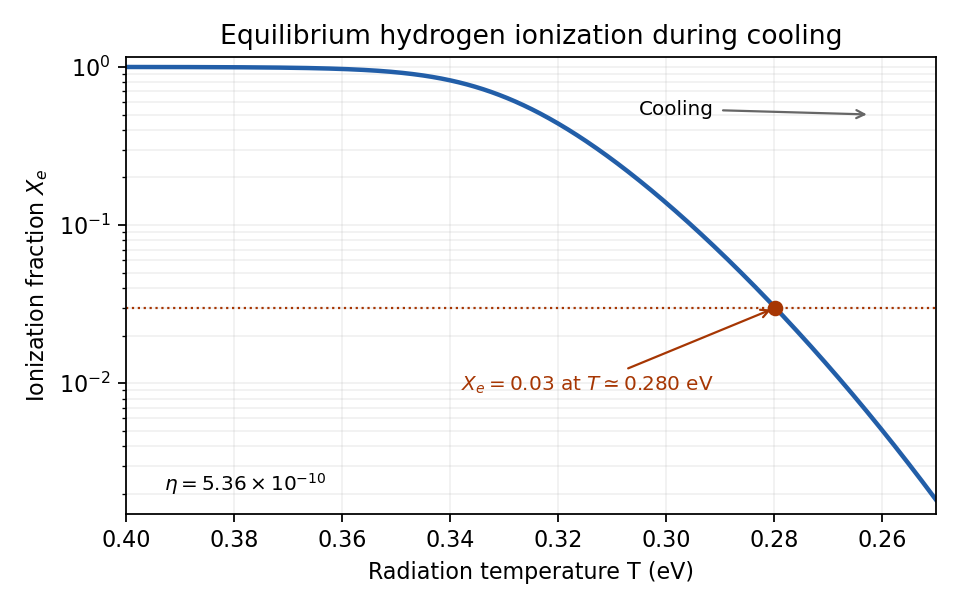
Hydrogen-only Saha ionization fraction during cooling, with the three-per-cent crossing near 0.28 electronvolts for baryon-to-photon ratio 5.36 times ten to the minus ten
. Details. 
Use the flat matter-only Einstein-de Sitter approximation for the distance-redshift relation, neglecting radiation corrections at cosmological recombination. Let be the cosmological recombination redshift. Adiabatic photon cooling gives . The Hubble rate is , so the comoving radial distance to last scattering isThe angular diameter distance is . A proper Hubble radius therefore subtends the small angleThis is the angular Hubble-radius scale in an Einstein-de Sitter universe; the present Hubble constant cancels.
Taking and the literal printed gives and radians, or degrees. As noted above, that present CMB energy is too large by ten. With the corrected , andwhich gives the familiar order-one-degree scale within the assumed cosmology. Using to mark a few-per-cent ionization fraction changes this only modestly. These numbers refer to the Hubble-radius scale, not its diameter. In a matter-only universe the particle-horizon radius is and would give twice the angle; the acoustic sound horizon is a different length again.
At linear order a coordinate displacement changes a metric perturbation by . Work in conformal time with , write and lower spatial indices with . Directly evaluating the Lie derivative of a covariant tensor field givesHere primes on mean conformal-time derivatives, while primes on label transformed components. Setting the transformed lapse and shift perturbations to zero requiresThese are first-order time equations. Their explicit local solutions areThus four coordinate functions can impose the four synchronous conditions in any regular perturbative patch. This is synchronous gauge fixing by coordinate displacement. The arbitrary spatial functions remain as residual gauge freedom; the conditions alone do not fix the coordinate system completely.
Geometrically, synchronous coordinates follow a congruence of freely falling observers launched normally from a spatial slice, using their proper time. This gives unit lapse and zero shift in cosmic time; conversion to background conformal time gives the displayed convention. “Always possible” is local: geodesic caustics or singularities can prevent a global synchronous chart. Such global obstructions do not invalidate local linear cosmological perturbation theory.
Use primes for conformal-time derivatives. The cold-dark-matter Cosmological Euler equation in synchronous gauge is , so multiplying by gives . ThereforeIn an expanding universe increases, damping any initial peculiar velocity as . During radiation domination , so the velocity scales as ; during matter domination , it scales as . This is the nonrelativistic limit of the physical-momentum redshift derived in Q1. It concerns the bulk velocity in the synchronous coordinate frame, not a growing peculiar velocity sourced in another gauge. A cold-matter rest-frame choice also removes the residual synchronous time displacement relevant to that component. The decay statement assumes expanding evolution and the pressureless, linear approximation used by the equation.
With negligible cold-dark-matter velocity, the synchronous perfect-fluid density equation gives . Differentiate and use the trace Einstein equation, taking the cold matter sound speed to vanish and its density to dominate:In a spatially flat matter-dominated universe, , , and the conformal Friedmann equation gives . HencePut . The indicial equation is . These two independent modes span the solution space, soEquivalently the growing mode is proportional to and the decaying mode to . The coefficients are set by initial data. Since synchronous gauge has residual coordinate modes, interpreting the density contrast physically requires fixing its residual freedom consistently, for example by the cold-matter rest frame and metric tensor integration convention; the mode equation alone is not a gauge-invariant observable.
The continuity and Cosmological Euler equation in synchronous gauge combine particularly simply. Differentiate and add :The velocity terms cancel by the Cosmological Euler equation in synchronous gauge, so this step does not require setting the initial velocity exactly to zero.
For subhorizon modes deep in radiation domination, take the rapidly oscillating radiation perturbation to be negligible in the averaged gravitational forcing. Also neglect the subdominant matter self-gravity to leading order in . With and , the resulting equation isIntegrating twice giveswhere the arbitrary reference time makes the logarithm dimensionless and can be absorbed into . This is logarithmic growth of matter perturbations during radiation domination.
The neglect of matter self-gravity is needed for the displayed form to be exact within the leading radiation-background approximation. Uniform radiation alone leaves a nonzero term if the cold-matter density is retained. Relative to , its coefficient is , small deep in the radiation era but not near equality. The Mészáros equation retains that effect in a matter-plus-radiation background; its solution basis tends to a constant and a logarithm at , recovering the present leading result. It connects smoothly to matter-era growth rather than allowing the logarithmic approximation to be extrapolated indefinitely.
Galaxy-scale modes enter the Hubble radius before matter-radiation equality. The earlier radiation forcing and horizon-entry matching ordinarily generate a nonzero logarithmic coefficient, even though subsequent oscillatory radiation forcing is small. A Fourier mode with entry time accumulates before equality. Across a large scale-factor range this factor need not be small, so treating the density contrast as exactly frozen would lose an important part of the galaxy-scale seed amplitude and its scale dependence. Growth is nevertheless much slower than in matter domination. This is the Mészáros effect, and the logarithmic matching contributes to the small-scale matter cold-dark-matter transfer function.
Articles by others on the same topic
There are currently no matching articles.