Past exam of the mathematics course of the University of Cambridge / 2013 / iii / Paper 70 (Sound Generation and Propagation)

Put ${\rho }^{\prime }=\rho -{\rho }_0$, and take the retarded acoustic Green function for ${\partial }_t^2-c_0^2{\nabla }^2$:This selects the causal, outgoing acoustic density perturbation, with no additional incoming homogeneous wave equation solution. Convolving the acoustic dipole forcing with this Green function and moving its spatial derivative outside the integral givesThe surface delta distribution converts the spatial integral to the moving surface. At fixed surface labels $(p,q)$, setThe radial Mach number enters the moving-surface retarded Jacobian, because $dr/d\tau =-\hat{r}\cdot v$ and henceLet ${\tau }^{\ast }$ be a root of the retarded time equationThe delta change-of-variable rule now givesHere $h_p{h}_q$ is the surface-area factor from the orthogonal surface coordinates. For a subsonic surface, $|v|<c_0$, the retarded equation is monotone in $\tau$ and has one root when the motion is defined for the required past times. For more general motion, sum the displayed contribution over all simple retarded roots. A root with $1-M_r=0$ requires a separate limiting treatment; the simple-root formula does not apply there.

In the Ffowcs Williams-Hawkings equation, the other source types are a surface acoustic monopole associated with acoustic thickness noise, and a volume acoustic quadrupole involving the Lighthill stress tensor. On an impermeable material surface, fluid and surface normal velocities agree. There is no through-surface mass-flux source; the remaining thickness source is $Q={\rho }_0{v}_n$. For a rigid body, the leading acoustic compact-source approximation to that source hasThus there is no leading net-volume acoustic monopole. To neglect thickness radiation beyond that leading cancellation, assume negligible volume displacement, as for ideal thin blades, or that its higher multipoles are small compared with the retained acoustic loading noise. Rigidity alone does not make a moving finite-volume body's local thickness source identically zero.

The volume acoustic quadrupole may be neglected for low Mach number motion when exterior turbulent or nonlinear stresses do not provide a competing strong source. We also assume small linear acoustics perturbations, a uniform reference sound speed, and negligible relevant viscous and entropy sources. These are source-strength approximations, particularly important if a loading contribution itself cancels by symmetry. Under them, the retained acoustic dipole is the force exerted by the object on the fluid, with the sign used in the previous solution.

Let $R=|x|$, $n=x/R$, and ${\tau }_0=t-R/c_0$. In the acoustic far field, $R$ is large compared with the object and $\omega R/c_0\gg 1$. For a source of size $\ell$ with $\omega \ell /c_0\ll 1$ and small surface Mach number, source-dependent delays and the Doppler factor can be neglected to leading order. The surface integral then contains just the total force $\mathcal{F}(\tau )={\int }_{S}FdS$. Differentiating its retarded time, rather than its $R^{-1}$ spreading factor, gives the radiating termThe sign follows from ${\partial }_{x_i}{\tau }_0=-n_i/c_0$. Differentiating $R^{-1}$ or the direction $n$ instead produces the lower-order near field. A constant total force does not radiate at this leading compact order.

The rotation introduces angular frequency $\Omega$ and, after combining the two blades, harmonics such as $2\Omega$. The acoustic compact-source approximation requires the propagation time $a/c_0$ to be small compared with ${\Omega }^{-1}$. ThusIt also bounds every blade element's Mach number by $\mu$. Consequently $|1-M_r|=1+O(\mu )$, and its leading value is one. The separate acoustic far field condition is $\Omega R/c_0\gg 1$.

Choose the positive rotation sense so that a first blade at phase $\alpha$ has radial and tangential unit vectorsIntegrating the given line force from $r=0$ to $a$ yields ${\mathcal{F}}_1=F{e}_{\varphi }(\Omega \tau )+D{e}_x$. Its axial component is constant, while ${\dot{\mathcal{F}}}_1=-F\Omega e_r$. Since $n=\cos \theta e_x+\sin \theta e_y$, the compact acoustic dipole sound from this blade isThe other blade has phase $\alpha +\pi$ and contributes the opposite rotating force. At a common compact retarded time, their total force is $2D{e}_x$, soThis cancellation calls for the next source-delay correction; it does not mean that the complete moving-source field vanishes.

Write $\alpha =\Omega {\tau }_0^{\ast }$ and $s=\sin \theta$, where ${\tau }_0^{\ast }=t-R/c_0$. Label the two arms by $\sigma =\pm 1$. Their positions are $y_{\sigma }=\sigma r{e}_r(\Omega {\tau }_{\sigma }^{\ast })$. To radiating far-field accuracy,The retarded time equation therefore gives, with ${\mu }_r=\Omega r/c_0$,For the first arm, $\sigma =1$, this is the requested phase expansion. The more explicit geometric error also makes the dimensional meaning of the printed $O(1/R)$ term clear.

Apply the Taylor theorem to the rotating line force. Since $d{e}_{\varphi }/d\alpha =-e_r$, its first two orders, expressed in a common reference frame, areAlso $v_{\sigma }=\sigma \Omega r{e}_{\varphi }(\Omega {\tau }_{\sigma }^{\ast })$, so the radial Mach number isThe absolute value causes no change of sign in this subsonic limit. Multiplying these two expansions before summing is essential: both the shifted force and the moving-surface retarded Jacobian contribute at the same order.

Denote the integrated numerator, including that Jacobian, by $\mathcal{B}$. Pairing the two blades cancels all terms odd in $\sigma$, including the first Doppler correction to the axial load. HenceThe factor $a/3$ comes from $a^{-2}{\int }_0^a{r}^{2}dr$. Only the time-dependent term radiates at order $R^{-1}$. Applying $-{\partial }_{x_i}$ to the integral now gives ${\rho }_{\mathrm{rad}}^{\prime }=(4\pi c_0^{3}R{)}^{-1}n\cdot {\partial }_t\mathcal{B}$, and thusThere are also nonradiating terms of order $R^{-2}$. Multiply by $c_0^2$ for the acoustic pressure. The stated coefficient uses the rotation convention fixed above; reversing the rotation reverses the corresponding signed load and phase convention.

This is a compact rotating two-blade loading source acting as an acoustic quadrupole. The compact total rotating force cancels, leaving the first spatial moment of the loading. Its two factors of the observer's projection into the rotor plane produce ${\sin }^2\theta$: there is no leading sound on the rotation axis and the density amplitude is maximal in the rotor plane. The configuration repeats after half a rotation, explaining frequency $2\Omega$. These statements concern amplitude; the corresponding acoustic intensity has a ${\sin }^4\theta$ factor.

If $F=0$, the displayed first-order contribution vanishes as well. For completeness, expanding the axial Jacobian to its next even order givesThe first remaining axial-load radiation is thenThus the constant axial total force does not produce the lower-order term, even though its moving spatial distribution can radiate at a higher order.

Use the prescribed harmonic convention $e^{i\omega t}$. For a propagating acoustic plane wave, let $k=(\omega /c_0)\cos \theta$ and $\ell =(\omega /c_0)\sin \theta >0$. The incident and reflected pressure amplitudes in the upper half-space have vertical factors $e^{i\ell y}$ and $e^{-i\ell y}$ respectively:The linear homentropic acoustic equations imply $i\omega {\rho }_0{v}_y=-{\partial }_y{p}^{\prime }$. At the surface, the normal velocity is therefore $\ell (R-A)/({\rho }_0\omega )=-V$, while the pressure amplitude is $P=A+R$. The surface acoustic impedance condition $P=ZV$ givesHere $Z_f$ is the normal acoustic impedance; the angle in this question is measured from the horizontal, not the normal. For a passive acoustic impedance, the mean power absorbed per unit area is $\frac{1}{2}\mathrm{Re}(P{V}^{\ast })=\frac{1}{2}\mathrm{Re}Z|V{|}^2\ge 0$. The four limiting cases have distinct meanings:

Define $k_0=\omega /c_0$ and use the outgoing acoustic square-root branchFor positive real frequency reached from below, $\gamma =i\sqrt{k_0^2-k^2}$ on the propagating interval and is positive real for $|k|>k_0$. The outgoing field in the lower fluid has pressure amplitude $B{e}^{\gamma y}$, since $y<0$. If $\eta =\hat{\eta }{e}^{i\omega t-ikx}$, the shared normal velocity is $i\omega \hat{\eta }$. The linear homentropic acoustic equations therefore giveThis lower-fluid wave is outgoing; no additional incoming sound is included in defining the impedance seen by the upper fluid.

Put $K_s=T{k}^2-m{\omega }^2$. The sheet's force balance gives $K_s\hat{\eta }=-P+B$, hence $P=({\rho }_0{\omega }^2/\gamma -K_s)\hat{\eta }$. Its prescribed downward velocity amplitude is $V=-i\omega \hat{\eta }$. Thus the tensioned-sheet acoustic impedance isThe first term is the lower fluid's normal acoustic impedance, and the second is the sheet's inertial and elastic-sheet tension response. For a real propagating angle, $Z_f={\rho }_0{c}_0/\sin \theta$.

At fixed nonzero frequency and fixed wavenumber, $m\to \infty$ gives $|Z|\to \infty$, a zero-velocity, in-phase reflecting boundary. At fixed $k\ne 0$, $T\to \infty$ gives the same reflection limit, but there is an important exception: elastic-sheet tension does not resist the spatially uniform mode $k=0$. At normal incidence, the impedance remains ${\rho }_0{c}_0+im\omega$ however large the elastic-sheet tension is. With $m=0$ this mode is transparent. By contrast, arbitrarily large mass resists even a spatially uniform oscillation. These fixed-frequency limits exclude a simultaneously tuned structural resonance.

If $m=T=0$, $Z=Z_f$ and $R=0$. The identical fluids are effectively joined across a massless, untensioned interface: pressure and normal velocity continue without reflection. This is the matched case, rather than the pressure-release case.

With no incoming wave, both fluids obey the outgoing acoustic square-root branch. Their surface pressure amplitudes areSubstitution in the sheet's force balance yields the dispersion relation for an acoustic membrane wave:The equivalent denominator $\Delta =\gamma (T{k}^2-m{\omega }^2)-2{\rho }_0{\omega }^2$ is useful away from the branch points $\gamma =0$. For real guided modes with $|k|>k_0$, this is the familiar added mass of an evanescent fluid layer formThe normal fields decay away from the sheet; continued by analytic continuation roots may describe radiating or leaky modes.

On $D=0$, $T{k}^2-m{\omega }^2=2{\rho }_0{\omega }^2/\gamma$, so the impedance from the preceding solution isThus the divergence of the reflection coefficient corresponds to a reflection pole of a fluid-loaded membrane. The prescribed incoming amplitude is zero, but a homogeneous fluid-sheet mode can have nonzero amplitude. This is a resonance or guided-mode pole of the analytic scattering problem, not arbitrarily large passive reflection at a real propagating angle. In particular, an undamped guided mode has an evanescent normal field and therefore a complex incidence angle in the plane-wave continuation. For real propagating incidence, $Z_f>0$ and the finite-mass, finite-tension sheet has a purely imaginary structural impedance, so its passive reflection remains bounded.

Use the Fourier transform pair $\hat{q}(k)=\int q(x)e^{ikx}dx$, $q(x)=(2\pi {)}^{-1}\int \hat{q}(k)e^{-ikx}dk$. The point force transforms to $F$. With the dispersion relation $D$ defined above, the sheet equation becomesThe point-force radiation from a fluid-loaded sheet is therefore represented exactly byThe causal contour and outgoing acoustic square-root branch are fixed first with $\mathrm{Im}\omega <0$, then continued to the desired real frequency. This prescription fixes how poles and the branch points are passed.

For the acoustic far field $x=r\cos \theta$, $y=r\sin \theta$, take $0<\theta <\pi$ bounded away from grazing and $k_{0}r\gg 1$. The method of steepest descent saddle point is $k_s=k_0\cos \theta$, with ${\gamma }_s=i{k}_0\sin \theta$. The supplied saddle point rule, including its $\sin \theta$ factor, gives, provided the contour deformation crosses no poles,A convenient simplification, free of division by $T$, isEquivalently, when $T\ne 0$,The expression printed in the PDF is missing sound-speed factors for general dimensional $c_0$. It agrees with this result if $c_0=1$ in fully normalized units; when $c_0$ is retained as an arbitrary sound speed, the numerator needs $c_0^{-3/2}$ and the structural term needs $T/c_0^2$ in the last form. These factors arise respectively from cylindrical spreading, the pressure-density relation, and $k_s=\omega \cos \theta /c_0$.

A direct countercheck is the transparent-sheet limit $m=T=0$. The sheet jump condition then gives ${\hat{p}}_{+}(k,0)=F/2$, so the saddle point rule requiresThe printed expression, interpreted continuously after multiplying out its structural factor, instead gives $F(2c_0{)}^{-1}\sqrt{\omega /(2\pi r)}\sin \theta$ times the same phase. It differs by a factor $c_0^{3/2}$; for example it is eight times too large when $c_0=4$. This limit also verifies the normalization of the corrected density field independently of the sheet's elastic-sheet tension.

To decide about poles, track the roots of $\Delta (k,\omega )$ on the chosen square-root sheet and deform the original causal contour to the steepest descent contour. A root contributes a residue exactly when it lies in the region swept out by that deformation; its sign is fixed by the contour orientation. Branch cuts must be retained throughout this comparison. Which roots are crossed can depend on observation angle, producing a change of the modal contribution when a pole meets the deformation boundary. A saddle point approaching a pole or a grazing endpoint requires an approximation uniform in that limit, rather than the isolated saddle point formula above.

The crossed poles are the free fluid-sheet modes of the preceding solution. Real subsonic roots represent evanescent acoustic surface waves carrying energy along the sheet, with normal decay; complex continuations represent leaky or radiating modes. Their residues must be added to the saddle point sound when the causal contour selects them. The specification “no poles contribute” is therefore a substantive condition on the contour, not permission to ignore zeros of the dispersion relation.

For the negative-flux Inviscid Burgers equation, the method of characteristics givesThe characteristic curve starting at ${\theta }_0$ therefore has $\theta ={\theta }_0-f_0({\theta }_0)z$, and henceFor smooth data this describes a single-valued classical solution as long as the characteristic flow map is invertible. Its Jacobian is $1-z{f}_0^{\prime }({\theta }_0)$; after characteristic crossing, one must instead select a weak solution with the appropriate entropy solution condition.

The conservation form is $f_z+G(f{)}_{\theta }=0$, with conservation law flux $G(f)=-f^2/2$. Integrating this scalar conservation law across a moving discontinuity, or differentiating its Heaviside representation as a distribution, yields the Rankine-Hugoniot conditionFor distinct one-sided limits it simplifies toThis jump-speed relation is exact for the Burgers conservation law; an additional entropy condition is needed to distinguish a physical compressive shock wave from an expansion discontinuity.

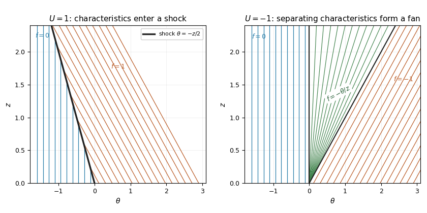
The step gives the Burgers Riemann problem with negative flux. If $U>0$, characteristic curves from the left have speed zero, while those from the right have speed $-U$: they converge. The entropy shock wave has speed $-U/2$ and thusCharacteristics enter this shock from both sides, since $0>-U/2>-U$.

If $U<0$, the right-hand speed $-U$ is positive and the two families separate. A smooth steep approximation to the initial step spreads into a rarefaction wave. In the fan, the self-similar characteristic curve relation is $-f=\theta /z$, givingThe endpoint values match continuously. The discontinuity moving at $-U/2$ would satisfy the jump condition even for $U<0$, but its characteristic curves leave the discontinuity and it fails entropy admissibility. For $U=0$ the solution is identically zero.

Set $q=\log \psi$ and use the sign-appropriate Cole-Hopf transformation $f=2\epsilon q_{\theta }$. Direct differentiation givesThus the heat equation ${\psi }_z=\epsilon {\psi }_{\theta \theta }$ implies the viscous Burgers equation with the required negative nonlinear sign. Conversely, vanishing of the Burgers residual makes the final quotient depend only on $z$, and a multiplicative time-dependent factor in $\psi$ removes it. The algebraic substitution works for any nonzero $\epsilon$ where $\psi \ne 0$.

For a forward dissipative initial-value solution, take $\epsilon >0$ and $z>0$. This is essential for the supplied heat kernel: at $\epsilon <0$, $z>0$, its real Gaussian integral diverges even for $\psi (0,\varphi )=1$. More generally that kernel requires $\epsilon z>0$. The physical viscosity convention selects the positive case; the mere condition $\epsilon \ne 0$ does not justify a forward Gaussian function formula.

Integrating ${\partial }_{\theta }\log \psi (0,\theta )=f_0(\theta )/(2\epsilon )$ gives a positive continuous initial factor, normalized asIts heat kernel convolution converges for both signs of $U$, since a Gaussian function dominates the one-sided exponential. DefineThe left half-line contributes $J(\theta )$; completing the square on the right half-line gives $e^{S}J(-\theta -Uz)$. ThusWhen differentiating, the two moving-endpoint Gaussian function terms cancel, becauseOnly ${\partial }_{\theta }{e}^S=(U/(2\epsilon ))e^S$ remains in the logarithmic derivative. The viscous Burgers step solution with negative flux is thereforeThe denominator is strictly positive, so $f$ lies between $0$ and $U$, irrespective of the sign of $U$. Its initial limits away from $\theta =0$ are the required step.

For the spatial limits, the Gaussian function tails must be compared with $e^S$; inspecting that exponential alone gives the wrong inference when $U<0$. As $b\to +\infty$, the complementary error function asymptotic givesAt $\theta \to +\infty$, $J(\theta )e^{-S}$ tends to zero even for $U<0$, because its quadratic decay dominates any exponential linear in $\theta$. Hence $\alpha e^{-S}\to 0$. At $\theta \to -\infty$, use the identity above to obtainwhile $J(\theta )$ approaches its full Gaussian integral. Thusfor both signs of $U$.

Since $J$ is strictly decreasing, $\alpha =1$ holds exactly when $\theta =-\theta -Uz$. At this point $S=0$, so the midpoint symmetry of a viscous Burgers step givesMore generally the exact symmetry is $f(z,-Uz-\theta )=U-f(z,\theta )$. For $U>0$, the midpoint follows the inviscid shock trajectory. For $U<0$, it is instead the center of an expanding fan, not a shock.

The vanishing viscosity approximation makes the comparison precise. For fixed $z>0$ and $U>0$, near $\theta =-Uz/2$ both tail integrals tend to the full Gaussian integral, so $\alpha \to 1$ andThe layer has width $O(\epsilon /U)$ and tends to the entropy shock, with value $U/2$ at its center. Outside it the limits are $0$ and $U$.

For $U<0$, inside $0<\theta <-Uz$ both Gaussian function tails have large positive lower limits. Their asymptotics giveOutside this interval the limits are $0$ on the left and $U$ on the right. Thus positive viscosity selects the rarefaction wave, including the same midpoint value as the inviscid fan. The two sign cases agree with the preceding entropy solution construction, while a negative diffusivity would not furnish this dissipative selection.