With , the chain rule gives . Since ,Substituting into the ordinary differential equation and multiplying by leaves , the harmonic oscillator equation. Its two independent real solutions are and . Undoing the change of variables givesThe constants are arbitrary real numbers. The reciprocal-coordinate reduction of a beam-type equation works on the entire positive half-line, where the coordinate transformation is invertible.
For continuously differentiable coefficients on a simply connected domain, the exactness condition is . Locally the same condition suffices without a global topological assumption. An exact first-order ordinary differential equation has a potential with and , so along a solution. Thus its implicit solution is . One local construction, on a rectangle about , isThe equality of cross derivatives verifies both required derivatives; on a simply connected domain one may use the corresponding path-independent integral of the exact differential form.
Here , and . Integrating with respect to gives . Matching gives , so take . The initial value sets . ThereforeThis is the requested explicit relation between the coordinates. Since , the implicit function theorem gives a unique local graph through the initial point, with slope .
Let the independent unit-step vectors be . The uniform distribution of each angle gives , while . With , expand the squared Euclidean norm:By independence, each cross term equals . HenceThis mean-square displacement of an isotropic planar random walk grows linearly even though the expected value of the displacement vector remains zero.
Write the countable supports as and the marginal masses as . Independence gives joint mass . Assuming finite expected values, absolute integrability is justified by Tonelli theorem:Consequently Fubini's theorem permits factorization of the signed sum, proving the expectation of a product of independent random variables:
The second claim holds as a general assertion with the additional hypothesis that the positive variables are integer-valued. For a nonnegative integer-valued , the pointwise identity and Tonelli theorem give the tail-sum formulaIf each is integer-valued, their product is too. Apply this identity to each factor and to the product, then use independence:Under the literal broader meaning of a discrete random variable, the second claim is false. Two independent constants are positive and discrete, but the left side is and the right side is . More generally the integer-indexed tail sum of a positive real-valued variable is , not . This is the integer-valued hypothesis in the tail-sum formula.
For and on an interval where , the logarithmic derivative substitution givesThe quadratic terms cancel. Multiplying by gives the linearization of a Riccati equation:Multiplying by a nonzero constant leaves unchanged. If , that substitution is undefined, but the original equation is already a first-order linear ordinary differential equation, solvable by an integrating factor.
For the particular equation, and the linear equation is . Use the PDF's logarithmic coordinate and write . The chain rule gives and , leaving . Thus , as also follows from the Euler-Cauchy equation. Recovering the Riccati equation solution yieldsThe initial value imposes ; choose . ThereforeThe denominator vanishes only at , and its numerator is then nonzero. This is a simple pole: . The maximal interval containing is ; the same expression on is a separate solution branch. These are poles of a Riccati solution from zeros of its linearizing solution.
Linearize about rest and a flat surface. An appropriate small-amplitude scaling has and , with gradients on fixed common length/time scales. Products such as and are then higher order. The linearized shallow water equations becomeDifferentiate the first with respect to time and substitute the second:The shallow-water dispersion relation therefore has a constant wave speed. In these equations is gravitational acceleration, despite the source's label “gravitational constant”; has units of speed squared.
In the characteristic coordinates, the chain rule gives and . HenceIntegrating this mixed derivative gives , a sum of oppositely traveling profiles. The initial data require and , soIntegrating the profiles and matching their total additive constant gives the D'Alembert formula with initial velocity:Here names the initial surface displacement, rather than the water velocity appearing in the original shallow water equations. The formula verifies both initial conditions directly.
With zero initial time derivative, the integral term in the D'Alembert formula vanishes. The Heaviside step function representation givesThe rectangular pulse splitting under the wave equation consists of two width-two pulses of height , moving left and right at speed . At they coincide and add to the initial height-one pulse. Before the overlapping interval has height one; after the two pulses are separated. Values exactly at the fronts depend on the chosen convention. Away from the fronts the equation holds classically, and across the fronts it holds as a weak solution of the wave equation.
Substitute and use to cancel the terms proportional to . The remaining ordinary differential equation isOn an interval where , divide through and put :Thus reduction of order givesA nonzero multiplicative constant gives an independent solution; adding a constant inside the integral adds a multiple of . The Wronskian is proportional to and is nonzero on the interval. The undivided equation remains meaningful at a zero of , but this integral representation then needs continuation rather than direct division.
Inspection gives in the degree-one Legendre differential equation. After division by , and . On either side of zero, reduction of order therefore givesA second solution is . Although is singular at zero, the product has a smooth continuation throughout . This illustrates reduction of order across a zero of the known solution. Since , , and , the required coefficients are . HenceThe ordinary differential equation has regular coefficients near zero, so the resulting initial-value solution is unique and the removable singularity in the intermediate representation causes no ambiguity.
Differentiate the mechanical energy and use the damped pendulum equation:The energy dissipation of a damped pendulum makes nonincreasing, rather than strictly decreasing at every instant: its derivative vanishes at turning points. It is constant along an equilibrium trajectory. Along every nonstationary trajectory it strictly decreases over any nonzero time interval, because a vanishing integral of over an interval would force an equilibrium there and hence everywhere by uniqueness.
The small-angle approximation replaces by , giving the damped harmonic oscillator equation . Its characteristic roots satisfy .
For , put ; the motion is underdamped:It oscillates with decaying amplitude. For , the repeated root gives critical damping:For , the motion is overdamped:Both real exponents are negative, so there is no oscillatory factor. The two constants are arbitrary in each case; these approximations require the displacement to remain small.
The phase plane system is , . Its equilibrium points are for every integer . At such a point the Jacobian matrix and characteristic equation areFor even , the equilibrium point is a stable focus for , with eigenvalues ; it is a stable node for , with two distinct negative real eigenvalues. The excluded value gives the repeated critical case.
For odd , the eigenvalues are . One is positive and one negative, so each is a saddle equilibrium for every . These classifications follow from the linearization of a dynamical system, since all the relevant eigenvalues have nonzero real part for . The even equilibria remain hyperbolic at too, although their linearization then has a repeated eigenvalue; that critical case is excluded from the requested classification.
For , the even equilibria are stable foci with eigenvalues , and the odd equilibria are saddle equilibria with eigenvalues . The local saddle directions are .
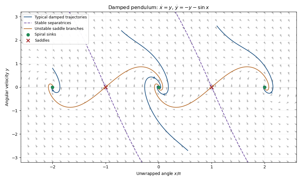
Phase portrait of a pendulum with unit damping, showing spiral sinks and the stable and unstable saddle branches
. The phase portrait shows clockwise spiraling into each even equilibrium: on its right-hand horizontal axis, the flow initially points down. The stable separatrices of the saddles divide attraction basins on the unwrapped angle axis, while the unstable branches flow into neighboring sinks. Initial conditions with enough mechanical energy can cross one or more potential crests before being captured. The curves repeat under . They are trajectories, not conservative energy contours: energy dissipation of a damped pendulum rules out nonconstant periodic orbits.
A probability space consists of a sample space , a sigma-algebra of events, and a probability measure satisfying:
- for every .
- .
- For pairwise disjoint events, .
For arbitrary events, Boole's inequality is . To prove it, replace each by . The are disjoint, have the same union, and satisfy . Countable additivity and monotonicity give . Finite unions are included by taking subsequent events empty.
Let be the th heads event. For every , the event of infinitely many heads lies inside . By the union bound, its probability is at most , which tends to zero. Thus the probability of infinitely many heads is . This is the First Borel-Cantelli lemma, and requires no independence of the coin tosses.
For the dice experiment there are ordered outcomes giving a sum of and giving , out of . Each trial therefore has , and irrelevant-outcome probability . By independence between trials, summing over the number of initial irrelevant outcomes givesThe geometric series also shows that one of the two relevant sums eventually appears almost surely. Equivalently, first-step analysis gives .
For , a Poisson distribution has mass for ; at it is concentrated at zero. Its moment-generating function isFor independent , the moment-generating function of their sum is the product, . Uniqueness of the moment-generating function near zero therefore gives . Repeating the argument gives when every parameter is one.
The displayed sequence is . The classical central limit theorem states that independent identically distributed variables with finite mean and nonzero finite variance have standardized sum converging in distribution to the standard normal distribution. Here , soConvergence of the distribution functions at the continuity point zero justifies the last step. This is the Poisson cumulative probability at its growing mean.
Assume , or use nonnegative with extended expectations. Let and . For , the discrete conditional expectation is . Therefore Fubini's theorem, or Tonelli theorem in the nonnegative case, gives the tower property of conditional expectation:Values of a conditional expectation on zero-probability conditioning events do not affect the sum. An unrestricted signed whose expectation is undefined is outside this assertion.
Write . The waiting time for two increments larger than dominates for and has mean , so is finite. Conditioning on the first increment, one step is always consumed; if that increment is below , the remaining independent sequence has the original law. Thus first-step analysis and the tower property of conditional expectation giveThis first makes continuous and then gives , with . Hence the uniform-sum crossing time below one hasAn independent explanation uses the tail-sum formula: for , since this region is an -dimensional simplex inside the unit cube. Summing from gives . In particular the strict-crossing convention gives almost surely and .
An exponential distribution of rate has density for and zero for , with survival probability . For , its memoryless property follows fromFor the minimum, independence gives . HenceThe density is zero for negative . The comparison probability follows from identical continuous laws and zero tie probability; directly it is . These are competing exponential clocks.
For the last density, substitute into the normalizing integral to obtain , the Gaussian integral. Equivalently, each variable has a gamma distribution with shape and rate one. Independence permits convolution of the densities. For ,Putting turns the integral into . ConsequentlyThis is also the additivity of independent gamma distributions with a common rate: their shapes add to one. Density values at the single endpoint zero are immaterial.
Articles by others on the same topic
There are currently no matching articles.