Squaring first avoids unnecessary expansion: , and squaring again gives the fourth power . In the polar form of a complex number, ; multiplying its complex argument by four gives the same negative-real result.
Write a nonzero complex number as . Matching modulus and complex argument gives and . Thus the four distinct fourth roots areThese angles differ by , so the values are distinct. Every further integer repeats one of them; this is multiplication by the fourth roots of unity.
The exponent in the PDF is . A complex exponential equals one precisely when its exponent is an integer multiple of : its real part must be zero, and its imaginary part must be a full rotation. Therefore for . Taking both square roots yields all solutionsThe first nonzero family corresponds to positive exponent index, and the second to negative index. Both signs are required.
For a real line , with , choose and . Direct multiplication gives , so every line has the required form with .
For a circle of centre and radius , expand its modulus equation:Thus the required circle parameters are . Conversely, completing the square in the circle form gives , which describes a genuine circle when . The complex conjugate terms make both equations real-valued.
An eigenvector of a matrix is a nonzero vector for which . The scalar is its eigenvalue. For a fixed eigenvalue, the zero vector together with all corresponding eigenvectors forms the eigenspace . The requirement prevents every scalar from being an eigenvalue merely because .
Expanding the characteristic polynomial givesSolving the three nullspace systems gives the eigenvalues and eigenspacesFor example, at the first two equations force and ; at they force and ; at they force .
Putting these eigenvectors in columns proves their linear independence:Hence is a diagonalizable matrix over the reals.
Call an index a peak if for every . If there are infinitely many peaks, list their indices increasingly. Each selected value is at least every later selected value, so this gives a nonincreasing subsequence.
If there are only finitely many peaks, choose an index beyond the last one. Every index from then onward has a later index with strictly larger value. Select these recursively: with . This gives an increasing subsequence. Neither complex argument requires the original sequence to be bounded. Every real sequence therefore has a monotone subsequence, as asserted by the monotone subsequence theorem.
Let . Its consecutive coefficient ratio isThe ratio test for the full terms therefore has limit : the series has absolute convergence when and its terms eventually grow in magnitude when . Thus the radius of convergence is . No boundary decision is needed to determine the radius of convergence.
This is a lacunary power series: the coefficient of is , while the other coefficients are zero. Along its nonzero coefficients,The factorial dominates ; for example for large already suffices for this limit. Hence the coefficient limsup in the Cauchy-Hadamard theorem is one. The radius of convergence is .
Directly, for the consecutive term ratio is , which tends to zero; for the term magnitudes are at least and fail to tend to zero. The factorial is the exponent of , not part of its coefficient.
The first coordinate of the vector triple product isThe other two coordinates follow by cyclically permuting the indices, proving the identity.
A point on the line has the form . Substituting in the plane equation gives . When the parameter, and therefore the intersection point, is unique. The vector triple product gives , so the unique intersection isFor the parallel case , the line is entirely in the plane if , and otherwise has no intersection. As usual, a genuine line and plane require nonzero direction and normal vectors. This is the line-plane intersection criterion.
The plane through has the constant normal coordinate . Since is a unit vector, the separation of these normal coordinates is a length. Every displacement joining the planes has this fixed normal component, so its length is at least its absolute value; a displacement parallel to attains that bound. Hence the distance between parallel planes isThe absolute value, present in the PDF, is necessary because distance is nonnegative.
Take points and with directions and . A common normal is , of length . The planes through the two lines with this common normal have separationThis is a lower bound for the distance between skew lines. It is attained at and : the two points are and , whose difference is perpendicular to both directions and has length . Thus the shortest distance is .
View a possible complex eigenvector using the Hermitian inner product. For a real symmetric matrix, , so is real. Since and , every eigenvalue is real.
For eigenvectors with distinct eigenvalues , symmetry givesso . In particular, real eigenvectors are orthogonal in the real dot product.
Use the permitted diagonalizability assumption to take bases of the real eigenspaces whose union spans . Apply the Gram-Schmidt process within each eigenspace. Its linear combinations remain eigenvectors of that same eigenvalue; vectors in different eigenspaces are already orthogonal. The resulting union is an orthonormal basis of eigenvectors, giving an orthogonal diagonalization of a real symmetric matrix.
If and , symmetry gives , proving necessity. Conversely, expand in the orthonormal basis from part (i), with . The zero-eigenvalue vectors span the kernel of a linear map. If is orthogonal to that kernel, then whenever , so the remaining coordinates can be solved independently.
For a nonzero eigenvalue and any associated nonzero eigenvector , symmetry gives . Thus the component vector along isFor the unit vectors , this coefficient is . Consequently the general solution isThis proves sufficiency as well as the claimed kernel criterion. If the compatibility condition fails, there is no solution; if it holds, the freedom is exactly an arbitrary kernel vector.
Reading the coefficients of the linear map givesUnder the inverse identification, the four standard real basis vectors map respectively to , , and in . Applying and taking real and imaginary parts therefore gives the columnsThus the real matrix isFor verification, write its blocks as , where is the planar rotation matrix. Block elimination gives . Therefore the determinant identity isThis is an instance of the realification determinant identity. The identification is real-linear; it is not an identification of complex vector-space dimensions.
Expanding the commutator immediately gives , , and . For its matrix trace, writeConsequently every matrix commutator is traceless: . This is the trace of a matrix commutator identity, valid for arbitrary square matrices over the complex numbers.
The conjugate transpose reverses multiplication. If and , thenThus the commutator is again a skew-Hermitian matrix. The order reversal is what produces the required minus sign.
For the map has the explicit formIts diagonal entries sum to zero and its conjugate transpose is its negative, because the three coordinates are real. Hence it is traceless and a skew-Hermitian matrix.
Direct multiplication of the given basis matrices yieldsThe reverse products give the negative commutators, and equal-index commutators vanish. Bilinearity then givesThus the cross product is represented by the commutator:This realizes the cross-product model of su(2) with exactly the normalization and cyclic orientation used here.
Every traceless skew-Hermitian matrix of size two has the formso it equals for . If , take . Otherwise choose a unit vector perpendicular to and set , . The vector triple product gives .
By part (iii), choosing and gives the required representationIn fact both factors can themselves be chosen as traceless skew-Hermitian matrices. The cross-product model of su(2) explains this geometric commutator construction.
Use , the derivative identity , continuity of cosine at zero, and . For , the mean value theorem gives for a point between zero and . Hence as . For , apply this with to obtain the limit . For every term is zero.
The additional bound and the same mean value theorem give . ThereforeThe right side is summable. By the comparison test for series the stated series has absolute convergence for every real .
Let . The geometric series from any starting index is bounded:Using summation by parts,Since the coefficients are nonincreasing and positive, the modulus is at most . The Cauchy criterion proves convergence for every . This is a direct proof of the Dirichlet test in this setting.
For , the imaginary parts of the convergent partial sums give convergence of the sine series at those angles. If , every sine term is zero. Hence the sine series converges for all real angles.
Take any inside the given open interval. Differentiability implies the continuity needed on , and the derivative is zero throughout it. The mean value theorem therefore gives . Since the two points were arbitrary, the function is constant on the interval.
For continuity at any , choose for a desired error . If , the stated bound gives . Thus is continuous, in fact uniformly continuous.
When , the difference quotient satisfiesTherefore the derivative exists at every point and is zero. Part (i) proves is constant. This is the lemma that Hölder exponent greater than one forces constancy; no differentiability was assumed in advance.
Apply the mean value theorem to on . It gives with . Both and are within of , soThis proves the endpoint secant-tangent approximation without any continuity assumption on . The continuity required by the theorem is only that of itself.
For , put and . The auxiliary function satisfiesRolle's theorem first gives a zero of strictly between zero and . Apply Rolle's theorem to between that zero and zero, where , to obtain a zero of . Continue in this way. The derivatives through order are continuous, since they are differentiable; hence every application is valid even if is not continuous. After applications there is strictly between zero and with .
But , so . Writing yields the Taylor formula with Lagrange remainderThe same construction using repeated applications of Rolle's theorem applies when , with intervals ordered from to zero. For the identity is immediate and any works. This proves the Taylor theorem with Lagrange remainder using only the allowed theorem and elementary differentiation.
From , differentiating successively gives and whenever those derivatives have been constructed. Starting with twice differentiability, this relation supplies the next two derivatives at each stage. Thus is infinitely differentiable, and its origin series isFor a fixed , both and are bounded on the compact interval between zero and , say by . Every higher derivative is one of these two functions. Taylor's theorem, with the remainder just proved, therefore bounds the order- remainder by , which tends to zero: its consecutive positive-term ratio is . Hence the series converges to for every real . It also gives by the usual hyperbolic-function series.
At any other centre , apply the proved origin result to , which also satisfies . Its even derivatives at zero are , and its odd ones are . ConsequentlyThis proves convergence at every centre without assuming that smoothness alone implies equality to a Taylor series.
For a bounded real function on , take a partition with nodes . Its lower Darboux sum and upper Darboux sum areThe function is Riemann integrable when ; their common value is its Riemann integral. Equivalently, for every some partition has . Indeed a common refinement of nearly extremizing upper and lower partitions proves necessity, while arbitrarily small gaps force equality of the two integrals. This is the Riemann integrability criterion.
A continuous function on a compact interval is bounded and uniformly continuous. Choose a mesh small enough that its oscillation on each subinterval is less than . Then ; using first makes the desired inequality strict. Thus every continuous function on is Riemann integrable.
For a nondecreasing function, the endpoint bounds show it is bounded. On the uniform partition into intervals, its Darboux sums satisfyFor a nonincreasing function apply the same calculation to , or use . Thus every monotone function on is Riemann integrable.
For the unheaded rational-weight example, each summand is nonnegative, and increasing only adds indices. Hence its sum is nondecreasing and lies between zero and one, including the separately specified value at zero. It is a left-continuous cumulative function of an atomic measure.
If and , the index appears in the sum at but not at . All other changes are nonnegative, so . This remains true for arbitrarily small positive , proving discontinuity at , including a right discontinuity at zero when that rational is encountered. Every interval of positive length contains such a rational in its interior. The discontinuities are therefore dense, although the function is Riemann integrable by the monotone-function result just proved.
More concretely, truncate after the first weights. The resulting finite sum of step functions is integrable, and the uniform tail is at most . This also proves integrability and gives, if its value is desired,The integral formula follows by integrating the finite sums and using the uniform tail bound. Here “every interval” has the usual nondegenerate-interval meaning; a singleton is not being asserted to contain a discontinuity.
With , the chain rule gives . Since ,Substituting into the ordinary differential equation and multiplying by leaves , the harmonic oscillator equation. Its two independent real solutions are and . Undoing the change of variables givesThe constants are arbitrary real numbers. The reciprocal-coordinate reduction of a beam-type equation works on the entire positive half-line, where the coordinate transformation is invertible.
For continuously differentiable coefficients on a simply connected domain, the exactness condition is . Locally the same condition suffices without a global topological assumption. An exact first-order ordinary differential equation has a potential with and , so along a solution. Thus its implicit solution is . One local construction, on a rectangle about , isThe equality of cross derivatives verifies both required derivatives; on a simply connected domain one may use the corresponding path-independent integral of the exact differential form.
Here , and . Integrating with respect to gives . Matching gives , so take . The initial value sets . ThereforeThis is the requested explicit relation between the coordinates. Since , the implicit function theorem gives a unique local graph through the initial point, with slope .
Let the independent unit-step vectors be . The uniform distribution of each angle gives , while . With , expand the squared Euclidean norm:By independence, each cross term equals . HenceThis mean-square displacement of an isotropic planar random walk grows linearly even though the expected value of the displacement vector remains zero.
Write the countable supports as and the marginal masses as . Independence gives joint mass . Assuming finite expected values, absolute integrability is justified by Tonelli theorem:Consequently Fubini's theorem permits factorization of the signed sum, proving the expectation of a product of independent random variables:
The second claim holds as a general assertion with the additional hypothesis that the positive variables are integer-valued. For a nonnegative integer-valued , the pointwise identity and Tonelli theorem give the tail-sum formulaIf each is integer-valued, their product is too. Apply this identity to each factor and to the product, then use independence:Under the literal broader meaning of a discrete random variable, the second claim is false. Two independent constants are positive and discrete, but the left side is and the right side is . More generally the integer-indexed tail sum of a positive real-valued variable is , not . This is the integer-valued hypothesis in the tail-sum formula.
For and on an interval where , the logarithmic derivative substitution givesThe quadratic terms cancel. Multiplying by gives the linearization of a Riccati equation:Multiplying by a nonzero constant leaves unchanged. If , that substitution is undefined, but the original equation is already a first-order linear ordinary differential equation, solvable by an integrating factor.
For the particular equation, and the linear equation is . Use the PDF's logarithmic coordinate and write . The chain rule gives and , leaving . Thus , as also follows from the Euler-Cauchy equation. Recovering the Riccati equation solution yieldsThe initial value imposes ; choose . ThereforeThe denominator vanishes only at , and its numerator is then nonzero. This is a simple pole: . The maximal interval containing is ; the same expression on is a separate solution branch. These are poles of a Riccati solution from zeros of its linearizing solution.
Linearize about rest and a flat surface. An appropriate small-amplitude scaling has and , with gradients on fixed common length/time scales. Products such as and are then higher order. The linearized shallow water equations becomeDifferentiate the first with respect to time and substitute the second:The shallow-water dispersion relation therefore has a constant wave speed. In these equations is gravitational acceleration, despite the source's label “gravitational constant”; has units of speed squared.
In the characteristic coordinates, the chain rule gives and . HenceIntegrating this mixed derivative gives , a sum of oppositely traveling profiles. The initial data require and , soIntegrating the profiles and matching their total additive constant gives the D'Alembert formula with initial velocity:Here names the initial surface displacement, rather than the water velocity appearing in the original shallow water equations. The formula verifies both initial conditions directly.
With zero initial time derivative, the integral term in the D'Alembert formula vanishes. The Heaviside step function representation givesThe rectangular pulse splitting under the wave equation consists of two width-two pulses of height , moving left and right at speed . At they coincide and add to the initial height-one pulse. Before the overlapping interval has height one; after the two pulses are separated. Values exactly at the fronts depend on the chosen convention. Away from the fronts the equation holds classically, and across the fronts it holds as a weak solution of the wave equation.
Substitute and use to cancel the terms proportional to . The remaining ordinary differential equation isOn an interval where , divide through and put :Thus reduction of order givesA nonzero multiplicative constant gives an independent solution; adding a constant inside the integral adds a multiple of . The Wronskian is proportional to and is nonzero on the interval. The undivided equation remains meaningful at a zero of , but this integral representation then needs continuation rather than direct division.
Inspection gives in the degree-one Legendre differential equation. After division by , and . On either side of zero, reduction of order therefore givesA second solution is . Although is singular at zero, the product has a smooth continuation throughout . This illustrates reduction of order across a zero of the known solution. Since , , and , the required coefficients are . HenceThe ordinary differential equation has regular coefficients near zero, so the resulting initial-value solution is unique and the removable singularity in the intermediate representation causes no ambiguity.
Differentiate the mechanical energy and use the damped pendulum equation:The energy dissipation of a damped pendulum makes nonincreasing, rather than strictly decreasing at every instant: its derivative vanishes at turning points. It is constant along an equilibrium trajectory. Along every nonstationary trajectory it strictly decreases over any nonzero time interval, because a vanishing integral of over an interval would force an equilibrium there and hence everywhere by uniqueness.
The small-angle approximation replaces by , giving the damped harmonic oscillator equation . Its characteristic roots satisfy .
For , put ; the motion is underdamped:It oscillates with decaying amplitude. For , the repeated root gives critical damping:For , the motion is overdamped:Both real exponents are negative, so there is no oscillatory factor. The two constants are arbitrary in each case; these approximations require the displacement to remain small.
The phase plane system is , . Its equilibrium points are for every integer . At such a point the Jacobian matrix and characteristic equation areFor even , the equilibrium point is a stable focus for , with eigenvalues ; it is a stable node for , with two distinct negative real eigenvalues. The excluded value gives the repeated critical case.
For odd , the eigenvalues are . One is positive and one negative, so each is a saddle equilibrium for every . These classifications follow from the linearization of a dynamical system, since all the relevant eigenvalues have nonzero real part for . The even equilibria remain hyperbolic at too, although their linearization then has a repeated eigenvalue; that critical case is excluded from the requested classification.
For , the even equilibria are stable foci with eigenvalues , and the odd equilibria are saddle equilibria with eigenvalues . The local saddle directions are .
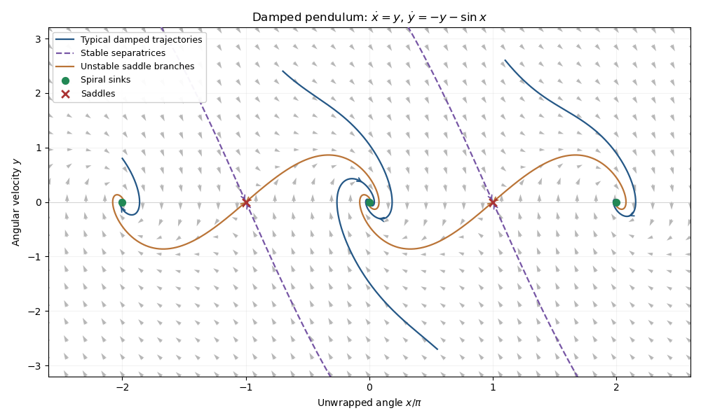
Phase portrait of a pendulum with unit damping, showing spiral sinks and the stable and unstable saddle branches
. The phase portrait shows clockwise spiraling into each even equilibrium: on its right-hand horizontal axis, the flow initially points down. The stable separatrices of the saddles divide attraction basins on the unwrapped angle axis, while the unstable branches flow into neighboring sinks. Initial conditions with enough mechanical energy can cross one or more potential crests before being captured. The curves repeat under . They are trajectories, not conservative energy contours: energy dissipation of a damped pendulum rules out nonconstant periodic orbits.
Articles were limited to the first 100 out of 235 total.
Articles by others on the same topic
There are currently no matching articles.