The integrating factor is , so . Integrating gives the general solutionThe particular solution is only defined up to a homogeneous solution. Subtract from it, absorbing that multiple into the arbitrary constant. The same family can then be writtenHolding fixed, the quotient tends to , the derivative of with respect to at . Thus the resonant family is . Direct differentiation gives , so it is the full general solution at resonance. This resonant exponential forcing in a first-order equation limit concerns a reparametrized family, not a fixed value of the original divergent constant . The initial condition gives , hence
The equilibrium points are . To obtain the other solutions of this separable differential equation without losing their signs, set on an interval where . Then , so . Therefore all real solutions areon intervals where . This family includes when . For a prescribed finite nonzero , and , so the solution exists for all future time. The cubic logistic differential equation hasThese are the only possible limits. The sign cannot change by uniqueness, and the denominator tends to one. A nonzero initial condition producing a constant solution is ; also works. The central equilibrium point is unstable and the two outer equilibrium points attract solutions from their respective half-lines.
For , the monotonicity of the logarithm and the uniform distribution giveFor the cumulative distribution function is zero. Differentiation gives the probability density function for , and zero elsewhere. The distribution is , with rate . This is inverse transform sampling of an exponential distribution.
Condition on the fair coin, taken independent of . For the squared uniform distribution, the cumulative distribution function of is on , giving probability density function . Reflection about gives the probability density function of as . Averaging the two conditional probability density functions produces this mixture model:There are no atoms at the endpoints; each integrable singularity contributes half the total mass. Equivalently the cumulative distribution function is on the interval.
Put , and . Because , the conditional probability inequality is equivalent to . But that same inequality gives , or . Thus positive association of two events is symmetric.
For the complement of an event, , andTherefore strictly repels ; equivalently . Both directions are stated because the wording switches the grammatical roles of attraction and repulsion. The substantive conclusion is the same: the conditional probabilities involving the complement are strictly smaller than their unconditional counterparts.
Introduce . The pendulum with quadratic damping is the autonomous planar systemIts equilibrium points are . Since the derivative of is zero at zero, the linearization of a dynamical system at each equilibrium point isAt an odd multiple of its eigenvalues are , so it is a saddle equilibrium; the stable and unstable tangents are and . At an even multiple the eigenvalues are . This linearization is a centre and does not decide the nonlinear stability. In particular it would be incorrect to infer a linear damped focus from this Jacobian.
For the full system the mechanical energy is a Lyapunov function near an even equilibrium point:A sufficiently small sublevel set is compact and contains only that equilibrium point. The only invariant motion with has and , hence is the equilibrium point itself. The LaSalle invariance principle proves asymptotic stability. Near it the trajectories turn clockwise and spiral inward, as the near-linear angular motion persists while energy decreases. Thus even equilibria are nonhyperbolic asymptotically stable spiral points; odd equilibria remain saddles.
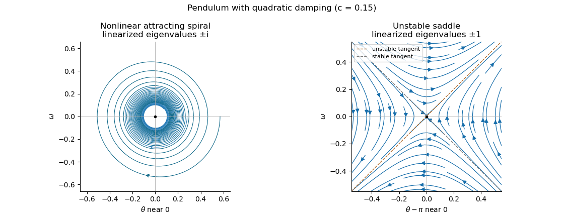
Local phase trajectories near a stable pendulum equilibrium and an unstable saddle with quadratic damping
. For explicit trajectories put on a branch where . The chain rule gives , so the two signs yield the first-order linear differential equations for , and for . Their integrating factors giveOnly portions with a nonnegative right-hand side are physical. At a turning point the constants of the two branches are matched using ; neither expression is one global trajectory through both signs. When they reduce to energy contours, with closed orbits around the even equilibrium points. For every , the quadratic damping destroys those closed orbits and makes the centres attracting spirals. Its effect is higher order in amplitude, so decay is weaker near rest than with linear damping. The saddle equilibria remain unstable, though their separatrices change shape.
The chain rule gives and . The coefficients of and are and . Their integer roots are and . Thus choose characteristic coordinates , , whose Jacobian determinant is . The coefficient of is , so the equation becomes , equivalently .
Integrating the transformed hyperbolic partial differential equation gives . Along the coordinates are , so the zero boundary condition gives for every real . Along they are , so , hence . The constants cancel and the unique resulting solution isIt directly satisfies both boundary conditions and .
Work on an interval where the change of variables is smooth and invertible, with . If , the chain rule gives and . Eliminating using the original second-order linear differential equation givesFor the real transformation as printed, take . Set , which is the Liouville transformation of a second-order equation. Differentiating twice makes the coefficient of cancel. Dividing by leavesThe additional term is exactly , as required.
On an interval with , choose and therefore up to a constant. Primes in the following expression mean derivatives with respect to . We have and , giving the WKB correction termNeglecting gives . Since , the WKB approximation isChanging the lower integration limit only rescales the constants. Small is the stated local approximation criterion; rapid variation or a turning point can invalidate it, and small local residual alone need not imply uniform accuracy over an arbitrarily long interval.
The printed hypothesis only says . If real on the interval, the printed square roots require a consistent complex branch. Equivalently a real WKB approximation isThis supplies the oscillatory interpretation for the negative- case instead of silently assuming that the original nonzero hypothesis means positive. Smoothness through the derivatives used above and absence of zeros are required locally.
The independence of eigenvectors for distinct eigenvalues ensures that such eigenvectors form a linearly independent set. For completeness, apply to a proposed relation . It leaves , so every . Thus the three eigenvectors form a basis over the relevant field and . Substitution into the linear system of ordinary differential equations gives ; linear independence implies . HenceA real matrix may have a complex conjugate pair of eigenvalues. In that case the calculation is over and conjugate coefficients yield real solutions; equivalently use real and imaginary parts of the complex modes. No unstated assumption that all three eigenvalues are real is needed.
The three linearly independent eigenvectors still form a basis, so the same coefficient calculation applies to this diagonalizable matrix matrix. The general solution isA repeated eigenvalue alone does not create a polynomial factor in time; that factor is needed only when a nontrivial Jordan block prevents a full eigenvector basis.
Suppose . Applying would give , contradicting linear independence of the two eigenvectors. Therefore the generalized eigenvector lies outside their span and is a basis. Write . Since , the linear system of ordinary differential equations givesSolving these equations gives , and . ThusThe length-two Jordan chain solution for the Jordan chain produces the mode. The three arbitrary constants span all initial data, so this is the full general solution.
Let and measure Lionel's fortune in unit stakes. This is gambler's ruin: the fortune moves by with probability and with probability , stopping at or . Let be the expected value of the absorption time starting at . It is finite: from any interior state, a run of wins or losses has a fixed positive probability of absorption within steps, giving a geometric bound on survival over successive blocks. First-step analysis therefore givesFor , the homogeneous solution of the recurrence is , and a particular solution is . Put . Imposing the two endpoint boundary conditions gives the expected duration of biased gambler's ruinConsequently the expected number of games isThe denominator and numerator have matching signs, so this is positive. As a check its continuous limit at is , the expected duration of symmetric gambler's ruin.
The proposed probability density function is nonnegative. To check its integral, put . The Gaussian integral can be evaluated by squaring and using polar coordinates:Since , and . Thus has the standard normal distribution. Completing the square in its moment-generating function gives, for every real ,Differentiation under the integral is justified near every finite by Gaussian decay. Expanding gives all moments:
To obtain the two-term bounds for Mills ratio, use . Integration by parts gives, for ,The positive remainder proves . A second integration by parts givesSubstitution and division by the strictly positive showThe last integral is strictly positive for every finite , proving . Both remainders are finite for every fixed positive ; the lower bound remains valid even when it is negative.
For a nonnegative random variable with finite expected value, and , Markov's inequality states . Indeed , and taking expected values proves the bound. For a random variable with mean and finite variance , apply Markov's inequality to at threshold . This proves Chebyshev's inequality:For independent and identically distributed random variables with finite mean and variance , the sample mean has expected value and variance . ThusThis is the weak law: , with the finite-variance hypotheses used in this direct deduction.
The more general weak law of large numbers needs only . To obtain that version, truncate . For fixed the bounded variables obey the result just proved. Their means tend to , while Markov's inequality bounds the probability that the two sample means differ by more than by . First take and then ; the integrable tail vanishes, proving the full integrable i.i.d. version as well.
Finally assume and . For every , implies , so Markov's inequality givesIf , the derivative of the right-hand side is , so its minimum is at . The Cantelli inequality follows:If , almost surely and the same bound is immediate. The bound is sharp: put mass at and the remaining mass at ; this has exactly the prescribed mean and variance.
Interpret random choice of coin as equal prior probabilities, and the tosses as independent conditional on the chosen coin. Let denote two heads. The conditional probabilities are and . For posterior coin selection from repeated tosses, Bayes theorem givesThe tosses need not be unconditionally independent, because the same hidden coin is used twice. If the coin-choice prior were instead , the answer would be ; equal choice gives the stated .
For nondecreasing uniform samples in the lottery, all ordered samples have equal probability by the discrete uniform distribution and independence. A nondecreasing sample is uniquely specified by its multiplicities , with . The stars and bars argument places separators among identical markers, giving multiplicity vectors. There is exactly one nondecreasing ordered sample for each such vector, so the probability isThis counts samples with ties correctly; multiplying a single strictly increasing count by would not handle the repeated values.
Articles by others on the same topic
There are currently no matching articles.