Write . Using the complex conjugate, the squared complex modulus on the left is . Squaring the equality and dividing by , which is nonzero, givesCompleting the square identifies the candidate circle:Its centre is on the real axis and its radius is in the complex plane.
It remains to exclude extraneous points introduced by squaring. On this circle, , so the original right-hand side satisfiesThus taking the nonnegative square root recovers the original equality at every point of the circle. This is a circle from an affine complex-modulus equation, with the sign check essential to the geometric conclusion.
Put . Since , the finite geometric series giveswhere the second equality multiplies numerator and denominator by . Taking imaginary parts gives the finite trigonometric sumTaking real parts of the same finite geometric series givesThe denominator is nonzero by the restriction on . Equivalently, these finite trigonometric sums are and , respectively.
Denote the four displayed matrices, from left to right, by . An orthogonal matrix has an orthonormal set of columns, equivalently . Direct column dot products give for . The first column of has squared Euclidean norm , so the third matrix is the unique nonorthogonal matrix.
For , the determinant is . A nonidentity orthogonal transformation of with determinant is a rotation: it has a fixed axis and restricts to a plane rotation on its orthogonal complement. Consequently is the rotation.
For , calculation givesA plane reflection fixes its entire plane, and therefore has eigenvalue . Since is invertible, is not a plane reflection. Thus is the combination of a rotation and a reflection. More explicitly, is an eigenvector with eigenvalue . On the perpendicular plane, is a rotation with , because . This gives a three-dimensional improper orthogonal transformation.
For , set . ThenThis reflection matrix reverses the normal and fixes every vector perpendicular to . Therefore is reflection in the plane . In particular, and . Finally represents none of the three listed orthogonal transformations, since each preserves the Euclidean norm.
For , the usual unit-circle area comparison, with angles measured in radians, gives . HenceThe cosine is a continuous function at zero, so the squeeze theorem yields the right-hand limit of a function . The quotient is even, so the left-hand limit of a function is the same. Thus the limit is .
For sufficiently close to zero, . Apply the mean value theorem to the logarithm between and : there is a point between these endpoints withAs from either side, , so this quotient tends to . The exponential function is continuous, and thereforeThe hypotheses of the mean value theorem hold because is continuous and differentiable for , with derivative .
For , the exponent lies in , and . ConsequentlyThe last inequality uses the positive-term power series for . The final bound tends to zero, so the squeeze theorem gives limit .
A complex power series with radius of convergence converges absolutely at every with and diverges at every with . This makes no general assertion at : boundary points must be examined separately. The series always converges at . If , no nonzero point lies in the convergence disk; if , the series converges absolutely throughout the complex plane.
If is the zero polynomial, every coefficient vanishes, so . Otherwise let be its degree and its leading coefficient. Since ,The ratio test therefore proves absolute convergence when . For , the terms do not tend to zero, so the series diverges. Thus the polynomial-coefficient power series has for every nonzero polynomial. In fact, it also diverges at every , because does not tend to zero, whether or .
The Cauchy-Schwarz inequality in isHere the Euclidean norm is induced by the dot product. If , the result is immediate. If , the squared Euclidean norm of the component of perpendicular to is nonnegative:Rearrangement proves the Cauchy-Schwarz inequality. Equality holds precisely when and are linearly dependent, including the cases of a zero vector.
Expanding the squared Euclidean norm and using the Cauchy-Schwarz inequality givesTaking nonnegative square roots gives the triangle inequality. Applying the triangle inequality once more gives
Subtract the two constraints to obtain . The Cauchy-Schwarz inequality gives . Since , division and squaring give the distance bound from two hyperplane constraintsIf and , the intersection is empty. If and , the constraints describe the same hyperplane. Its points satisfy , with equality at . The fraction involving is undefined in this case and cannot be used.
If , both equations are satisfied by every when , and otherwise there is no solution. These degenerate cases distinguish an inconsistent constraint from a repeated one.
Apply the triangle inequality to the path from through to :This is one direction of the reverse triangle inequality. A second application of the triangle inequality, this time through , givesThe resulting four-point triangle inequality follows without any assumptions on coincidences among the four points.
Write a vector in the domain as . The first and third equations defining the kernel of a linear map imply . Substitution into the second equation then givesFor , this forces , and . HenceThe kernel of a linear map has dimension one, so the rank-nullity theorem gives rank three and proves the assertion about the image of a linear map. Alternatively, the minor formed from columns has determinant , including a nonzero value at .
For , the parameters are free and , . ThusThe third row is the first row minus the second. The image of a linear map is therefore contained in . The first and third columns, and , are linearly independent, so the matrix rank is two and this containment is equality:This is the sole kernel jump in a parameter-dependent linear map; there is no further exceptional case at .
Let be the standard basis and define . By linearity,Thus every linear functional has this form. Its representing vector is unique because evaluating at each gives .
For the prescribed kernel of a linear map, the third listed vector is the first minus the second, so it adds no independent constraint. The first two requireTaking and gives , . Consequently all possible representing vectors areConversely, every such vector is perpendicular to each of the three prescribed vectors, so its linear functional vanishes on them. This also includes the zero linear functional.
The characteristic polynomials, in the convention , areSolving the eigenvalue equations gives the complete eigenspacesEvery nonzero vector in a listed eigenspace is an eigenvector, and these are all the eigenvectors. For , the repeated eigenvalue has a two-dimensional eigenspace; for , all three eigenvalues are simple. The three displayed generating vectors form a basis because their column matrixhas determinant . Thus both matrices are diagonalizable, with diagonal entries for and for in this basis.
Suppose and for an invertible and diagonal matrices . Since diagonal matrices commute,Therefore simultaneous diagonalization implies commutation. This argument works over either or and explains why simultaneous diagonalization produces commuting operators.
Let with . Commutation givesThus belongs to the eigenspace , with the zero vector allowed. Since has distinct eigenvalues, each eigenspace is one-dimensional. Hence for some scalar . This is the fact that commuting maps preserve eigenspaces.
The standard linear independence theorem for eigenvectors belonging to distinct eigenvalues supplies a basis of eigenvectors of . The preceding argument makes every one an eigenvector of as well. Their column matrix therefore simultaneously diagonalizes and . This is simple spectrum gives simultaneous diagonalization.
For real matrices, this conclusion always holds over ; a real common basis follows when the distinct eigenvalues of are real. Real matrix entries alone do not ensure a real eigenbasis: a quarter-turn of , with , has eigenvalues . The matrices in this question have real spectra, so their common basis is real.
Direct multiplication givesTake and in the preceding result: has the three distinct eigenvalues and the matrices commute. The common eigenbasis from part (i) givesIndeed and , and . These equalities directly verify the simultaneous diagonalization.
For the standard complex inner product, . Using the conjugate transpose and the defining equality for a normal matrix,Both norms are nonnegative, so for every .
Set . Its conjugate transpose is , soSince is a normal matrix, the two products coincide. Therefore is normal for every complex .
If , then is a normal matrix by part (ii), and . Part (i), applied to , yields . ThusThe nonzero vector is consequently an eigenvector of the conjugate transpose with eigenvalue . This adjoint eigenvector identity for a normal matrix will also determine the special spectral restrictions below.
The adjoint eigenvector identity for a normal matrix gives . HenceAs , . Thus eigenvectors in distinct eigenspaces of a normal matrix are orthogonal in the complex inner product.
Start with the assumed basis of eigenvectors, grouping them by eigenvalue. In each eigenspace, apply the Gram-Schmidt process, which replaces a linearly independent list by an orthonormal list with the same span. Every new vector stays within that eigenspace, since an eigenspace is a vector subspace.
By part (iv), different eigenspaces are orthogonal. The combined lists therefore form an orthonormal basis of the entire space, still consisting of eigenvectors. Let have these vectors as columns. Then is a unitary matrix, soThis gives the required unitary diagonalization of a normal matrix, including repeated eigenvalues.
For a Hermitian matrix, , so and is a normal matrix. If with , part (a)(iii) gives . Since also , we obtain . Thus every eigenvalue is real.
For a skew-Hermitian matrix, , so both and equal . It is therefore a normal matrix. On an eigenvector with eigenvalue , part (a)(iii) givesThus , and every eigenvalue lies in , including the possible eigenvalue zero.
For a unitary matrix, , so both defining products for a normal matrix are . The matrix is invertible, hence no eigenvalue is zero. If , then , while part (a)(iii) gives . Therefore , andThus all eigenvalues have unit modulus.
Since , shifting an index yields the summation by parts identityThe sum on the last line is empty when , so the identity also covers that case.
The series with a bounded monotone multiplier converges. Here is a proof that also permits conditional convergence. Choose with . The Cauchy sequence criterion for the convergent series ensures that, for any and sufficiently large , all the partial tails satisfy . Apply summation by parts to these partial tails:Since the multiplier is a monotone sequence, . ConsequentlyTaking proves that the weighted partial sums form a Cauchy sequence, and hence converge. This is a special case of bounded-variation multipliers of a convergent series.
The series also converges. The multiplier need only be monotone eventually, since a finite initial segment cannot affect convergence. For ,Thus decreases for ; it is bounded and tends to , because . Apply the proved multiplier result to the tail beginning at . The fact that the first few values are not monotone causes no difficulty.
We use the Bolzano-Weierstrass theorem: every bounded real sequence has a convergent subsequence. If were unbounded on , there would be with . The Bolzano-Weierstrass theorem gives a subsequence , and the closed interval contains . Since is a continuous function, , contradicting . Thus is bounded.
Let . By the definition of the supremum, choose with . Again the Bolzano-Weierstrass theorem gives . Continuity yields . Applying the same argument to gives a point where attains its infimum. Therefore both the supremum and the infimum are attained. This proves the extreme value theorem for a closed bounded interval.
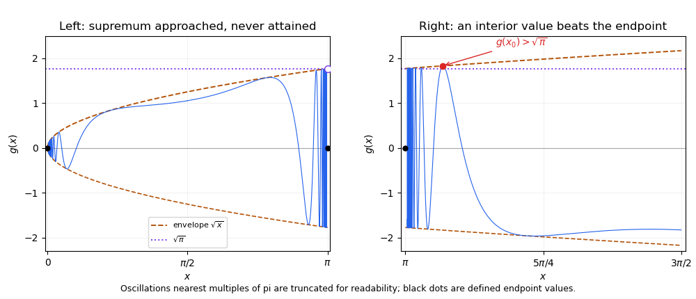
Away from integer multiples of , the function is a composition of continuous functions. At zero, the bound gives by the squeeze theorem. This is oscillation multiplied by a vanishing amplitude.
Fix and set and . Then , , andSo is discontinuous at every nonzero integer multiple of . Its set of continuity points is
On , for , while . With as above, . Consequently the supremum is and is not attained. This illustrates that supremum can fail to be attained at an oscillatory endpoint.
On , set . It lies strictly inside the interval, and , so . Choose . On ,On , is a continuous function, so the extreme value theorem gives a maximum there, at least . It exceeds every value on the discarded interval. Therefore does attain its supremum on . This is the interior-value criterion for an attained maximum.
The intermediate value theorem says that if is a continuous function, then every value between and is attained at some point of .
Endpoint values are already attained. Suppose and define . It is nonempty and bounded above, so exists. Continuity at ensures that contains points to the right of , and continuity at ensures that no point sufficiently close to belongs to . Hence .
By the definition of the supremum, there are points of approaching . If , continuity would exclude all such nearby points from , a contradiction. If , continuity would put some point to the right of in , again a contradiction. Therefore . When , apply this argument to . This proves the intermediate value theorem in all cases.
For a chord of length , consider the continuous function on . Since ,An endpoint zero already supplies the chord. Otherwise the endpoint values have opposite signs, so the intermediate value theorem supplies at some . Thus a horizontal chord of length exists.
For each integer , define on . The sampled differences telescope:If any sampled value is zero, it gives the required chord. Otherwise there must be both a positive and a negative sampled value. The intermediate value theorem, applied between their sample points, then gives . Hence a horizontal chord of length exists for every positive integer ; for , the endpoint chord itself suffices. This proves the horizontal chord of reciprocal-integer length result, without restricting to powers of two.
For a partition , write and for the upper Darboux sum and lower Darboux sum. The Riemann integrability criterion for bounded is that for every some partition satisfies . Thus if the gaps for tend to zero, the Riemann integrability criterion immediately proves that is Riemann integrable.
Conversely, suppose is Riemann integrable, and choose a fixed partition with . Let be the number of its interior division points and choose with . Call a cell of bad when its interior contains a division point of . There are at most bad cells, and their total length is at most .
Every other cell lies in a single cell of , so its oscillation is no larger than that of the containing cell. Summing the contributions of these good cells gives at most , while each bad cell has oscillation at most . Therefore the finite bad-cell estimate for Darboux sums givesFor large enough , the right-hand side is less than . This proves the uniform-mesh Darboux criterionThis argument does not assume that the partitions are nested; in general they are not.
For the composition, takes values in . Since is continuously differentiable, the extreme value theorem bounds both and on that interval. In particular, let . The mean value theorem states that a function continuous on the interval between and differentiable in its interior satisfies for some intermediate . HenceOn each partition cell, this bounds the oscillation of by times the oscillation of , whether or not the local extrema are attained. It follows thatThe composition is bounded, so the proved uniform-mesh Darboux criterion applies. Thus is Riemann integrable. The reusable fact is Lipschitz composition preserves Riemann integrability; continuous differentiability supplies the required bound on the range of .
The integrating factor is , so . Integrating gives the general solutionThe particular solution is only defined up to a homogeneous solution. Subtract from it, absorbing that multiple into the arbitrary constant. The same family can then be writtenHolding fixed, the quotient tends to , the derivative of with respect to at . Thus the resonant family is . Direct differentiation gives , so it is the full general solution at resonance. This resonant exponential forcing in a first-order equation limit concerns a reparametrized family, not a fixed value of the original divergent constant . The initial condition gives , hence
The equilibrium points are . To obtain the other solutions of this separable differential equation without losing their signs, set on an interval where . Then , so . Therefore all real solutions areon intervals where . This family includes when . For a prescribed finite nonzero , and , so the solution exists for all future time. The cubic logistic differential equation hasThese are the only possible limits. The sign cannot change by uniqueness, and the denominator tends to one. A nonzero initial condition producing a constant solution is ; also works. The central equilibrium point is unstable and the two outer equilibrium points attract solutions from their respective half-lines.
For , the monotonicity of the logarithm and the uniform distribution giveFor the cumulative distribution function is zero. Differentiation gives the probability density function for , and zero elsewhere. The distribution is , with rate . This is inverse transform sampling of an exponential distribution.
Condition on the fair coin, taken independent of . For the squared uniform distribution, the cumulative distribution function of is on , giving probability density function . Reflection about gives the probability density function of as . Averaging the two conditional probability density functions produces this mixture model:There are no atoms at the endpoints; each integrable singularity contributes half the total mass. Equivalently the cumulative distribution function is on the interval.
Put , and . Because , the conditional probability inequality is equivalent to . But that same inequality gives , or . Thus positive association of two events is symmetric.
For the complement of an event, , andTherefore strictly repels ; equivalently . Both directions are stated because the wording switches the grammatical roles of attraction and repulsion. The substantive conclusion is the same: the conditional probabilities involving the complement are strictly smaller than their unconditional counterparts.
Introduce . The pendulum with quadratic damping is the autonomous planar systemIts equilibrium points are . Since the derivative of is zero at zero, the linearization of a dynamical system at each equilibrium point isAt an odd multiple of its eigenvalues are , so it is a saddle equilibrium; the stable and unstable tangents are and . At an even multiple the eigenvalues are . This linearization is a centre and does not decide the nonlinear stability. In particular it would be incorrect to infer a linear damped focus from this Jacobian.
For the full system the mechanical energy is a Lyapunov function near an even equilibrium point:A sufficiently small sublevel set is compact and contains only that equilibrium point. The only invariant motion with has and , hence is the equilibrium point itself. The LaSalle invariance principle proves asymptotic stability. Near it the trajectories turn clockwise and spiral inward, as the near-linear angular motion persists while energy decreases. Thus even equilibria are nonhyperbolic asymptotically stable spiral points; odd equilibria remain saddles.
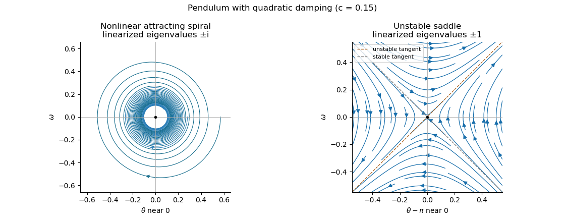
Local phase trajectories near a stable pendulum equilibrium and an unstable saddle with quadratic damping
. For explicit trajectories put on a branch where . The chain rule gives , so the two signs yield the first-order linear differential equations for , and for . Their integrating factors giveOnly portions with a nonnegative right-hand side are physical. At a turning point the constants of the two branches are matched using ; neither expression is one global trajectory through both signs. When they reduce to energy contours, with closed orbits around the even equilibrium points. For every , the quadratic damping destroys those closed orbits and makes the centres attracting spirals. Its effect is higher order in amplitude, so decay is weaker near rest than with linear damping. The saddle equilibria remain unstable, though their separatrices change shape.
The chain rule gives and . The coefficients of and are and . Their integer roots are and . Thus choose characteristic coordinates , , whose Jacobian determinant is . The coefficient of is , so the equation becomes , equivalently .
Integrating the transformed hyperbolic partial differential equation gives . Along the coordinates are , so the zero boundary condition gives for every real . Along they are , so , hence . The constants cancel and the unique resulting solution isIt directly satisfies both boundary conditions and .
Work on an interval where the change of variables is smooth and invertible, with . If , the chain rule gives and . Eliminating using the original second-order linear differential equation givesFor the real transformation as printed, take . Set , which is the Liouville transformation of a second-order equation. Differentiating twice makes the coefficient of cancel. Dividing by leavesThe additional term is exactly , as required.
On an interval with , choose and therefore up to a constant. Primes in the following expression mean derivatives with respect to . We have and , giving the WKB correction termNeglecting gives . Since , the WKB approximation isChanging the lower integration limit only rescales the constants. Small is the stated local approximation criterion; rapid variation or a turning point can invalidate it, and small local residual alone need not imply uniform accuracy over an arbitrarily long interval.
The printed hypothesis only says . If real on the interval, the printed square roots require a consistent complex branch. Equivalently a real WKB approximation isThis supplies the oscillatory interpretation for the negative- case instead of silently assuming that the original nonzero hypothesis means positive. Smoothness through the derivatives used above and absence of zeros are required locally.
The independence of eigenvectors for distinct eigenvalues ensures that such eigenvectors form a linearly independent set. For completeness, apply to a proposed relation . It leaves , so every . Thus the three eigenvectors form a basis over the relevant field and . Substitution into the linear system of ordinary differential equations gives ; linear independence implies . HenceA real matrix may have a complex conjugate pair of eigenvalues. In that case the calculation is over and conjugate coefficients yield real solutions; equivalently use real and imaginary parts of the complex modes. No unstated assumption that all three eigenvalues are real is needed.
The three linearly independent eigenvectors still form a basis, so the same coefficient calculation applies to this diagonalizable matrix matrix. The general solution isA repeated eigenvalue alone does not create a polynomial factor in time; that factor is needed only when a nontrivial Jordan block prevents a full eigenvector basis.
Suppose . Applying would give , contradicting linear independence of the two eigenvectors. Therefore the generalized eigenvector lies outside their span and is a basis. Write . Since , the linear system of ordinary differential equations givesSolving these equations gives , and . ThusThe length-two Jordan chain solution for the Jordan chain produces the mode. The three arbitrary constants span all initial data, so this is the full general solution.
Let and measure Lionel's fortune in unit stakes. This is gambler's ruin: the fortune moves by with probability and with probability , stopping at or . Let be the expected value of the absorption time starting at . It is finite: from any interior state, a run of wins or losses has a fixed positive probability of absorption within steps, giving a geometric bound on survival over successive blocks. First-step analysis therefore givesFor , the homogeneous solution of the recurrence is , and a particular solution is . Put . Imposing the two endpoint boundary conditions gives the expected duration of biased gambler's ruinConsequently the expected number of games isThe denominator and numerator have matching signs, so this is positive. As a check its continuous limit at is , the expected duration of symmetric gambler's ruin.
The proposed probability density function is nonnegative. To check its integral, put . The Gaussian integral can be evaluated by squaring and using polar coordinates:Since , and . Thus has the standard normal distribution. Completing the square in its moment-generating function gives, for every real ,Differentiation under the integral is justified near every finite by Gaussian decay. Expanding gives all moments:
To obtain the two-term bounds for Mills ratio, use . Integration by parts gives, for ,The positive remainder proves . A second integration by parts givesSubstitution and division by the strictly positive showThe last integral is strictly positive for every finite , proving . Both remainders are finite for every fixed positive ; the lower bound remains valid even when it is negative.
Articles were limited to the first 100 out of 229 total.
Articles by others on the same topic
There are currently no matching articles.