Work on a filtered probability space . A submartingale is a real-valued stochastic process satisfying the following three conditions: is -measurable, , andThus it is adapted, has integrable random variables at every time, and its conditional expected next value is at least its current value. Repeated conditioning gives for every . The inequality concerns conditional expectation; individual sample paths need not increase. If no filtration is specified, the definition can be applied to the natural filtration generated by the process.
The almost sure submartingale convergence theorem says that if a submartingale satisfiesthen there is an integrable random variable such thatIndeed the positive-part bound also bounds the negative parts, since ; the theorem gives a finite limit. In particular, the martingale convergence theorem applies to any martingale with .
For a nonnegative martingale, supplies this bound automatically. Its limit obeys by the Fatou lemma. Almost sure convergence alone need not preserve the expectation or give convergence in L1. Uniform integrability is the additional condition that supplies convergence in L1 and the identity .
Take independent and identically distributed random variables with the Bernoulli distribution of parameter , and their natural filtration. SetThe event at is the whole sample space. Independence givesso this is a nonnegative martingale; it is integrable with . The first zero among the is almost surely finite, since the probability of having only ones through time is . After that first zero, every is zero. Hence the almost sure limit is zero:This fair-coin doubling martingale also exhibits failure of uniform integrability: convergence in L1 would force the expectations to converge to zero.
Let be the natural filtration of the random walk on a graph. For a bounded harmonic function on a graph, the transition rule and the Markov property giveThus is a bounded martingale. The martingale convergence theorem gives a finite almost sure limit .
On the probability-one recurrence event, every vertex is visited along a sequence . Along that sequence , while convergence of the whole sequence forces . Therefore every pair of vertices has the same value. This is the bounded harmonic function theorem on a recurrent graph:Recurrence makes each vertex value a subsequential limit of the same convergent martingale. A connected locally finite graph is countable, since it is the union of its finite distance balls, so these almost sure assertions can also be combined by a countable intersection. The one-vertex case is immediate.
Write for the martingale difference sequence. Bounded increments mean that one deterministic satisfies for every , almost surely. Then and, for ,The increments are uncorrelated random variables, uniformly bounded in . Applying the supplied strong law for uniformly L2-bounded uncorrelated random variables gives almost surely. Also , because is finite almost surely. Therefore a martingale with bounded increments has zero linear growth:This is the strong law for martingales with bounded increments.
For the submartingale, let and define its predictable drift and compensator byThis is the Doob decomposition in discrete time. The process is a martingale. Since , we have , so . The result just proved gives almost surely, and . Consequently the strong law for submartingales with bounded increments isThe compensator may grow, so the conclusion is a lower bound rather than a claim of convergence to zero.
For each deterministic , use the nonnegativity and the martingale property to obtainA nonnegative random variable with zero expectation is zero almost surely. Hence almost surely on . Intersecting these probability-one statements over all makes them hold simultaneously, and induction givesZero is absorbing for a nonnegative martingale. This is the absorption at zero of a nonnegative martingale. On the assertion has no finite-time requirement. No unbounded-time use of the optional stopping theorem is needed.
The time is a stopping time, because . Apply the optional stopping theorem to the bounded time :On the stopped value is at least , and elsewhere it is nonnegative. Letting gives the maximal bound for a nonnegative martingale:Stop at a bounded time first, then pass to the increasing event. This avoids assuming uniform integrability of the original process. For , and the bound simply says .
The overshoot hypothesis as printed cannot hold for every . For , and ; choosing contradicts . The intended and sufficient assumption is the overshoot bound for , on the event . We use those thresholds below; when , the requested stopped-time bound is trivial because .
Fix and set . By part (a), the stopped martingale satisfies : before stopping it is below , at it is zero, and at the assumed overshoot bound applies. Thus the square of this stopped process is integrable. For ,The event is -measurable and contained in . Conditional expectation of the linear term is zero, while the variance assumption makes the remaining conditional expectation nonnegative. The stopped increments here are bounded by the stopping and overshoot bounds, so all conditional expectations are legitimate. ConsequentlySince , we have . Bounded-time optional stopping theorem also gives , soApply the monotone convergence theorem to . This proves the stronger estimate and hence the requested absorption-time bound from conditional variance and overshoot:In particular this stopping time is finite almost surely. For , and is a constant submartingale, while the stopping-time expectation is zero.
If , either , or both stopping times exceed . Therefore the maximal bound for a nonnegative martingale and the Markov inequality give, for ,The right-hand side is minimized at . Whenever the claimed bound is nontrivial, , this choice has and is allowed under the corrected overshoot hypothesis. Substituting gives the square-root tail bound for martingale absorption:When the displayed upper bound is at least one, the inequality follows from . This handles every without using the impossible small-threshold hypothesis.
Let and let the cumulant-generating function and its Legendre transform beUnder the permitted assumption that is finite everywhere, the right-tail form of the Cramér theorem is, for ,Use . The restriction to nonnegative parameters is valid on this side of the mean: convexity gives , so negative parameters cannot improve the value zero available at . For , the right-tail probability tends to one by the strong law of large numbers, so its logarithmic rate is zero; it is not generally .
The full large deviation principle bounds probabilities of closed sets from above and open sets from below with rate . For the displayed tail equality, a possible finite upper endpoint also needs attention. If , then at the event requires every summand to equal ; its probability is , and . The identity follows by taking in . Above , both sides have infinite rate. The theorem describes exponential decay, including endpoints and impossible events.
For every , the Markov inequality and independence give the Chernoff boundOptimize over nonnegative . For , part (a) identifies this supremum with , yielding the finite- estimateIf , use parameters with arbitrarily large ; the probability must then be zero. Taking the logarithmic upper limit proves the upper bound in the Cramér theorem:For , the nonnegative-parameter supremum is zero, giving the correct trivial tail-rate upper bound. Exponential Markov bounds and the product moment-generating function supply the entire upper-bound argument.
Write . The hypothesis implies and rules out a constant random variable. In particular . The cumulant-generating function is strictly convex, since its second derivative is the positive variance under exponential tilting, and , as .
If , there is a unique with , and the Legendre transform gives . ThusIf , use differentiability at zero: , so for some sufficiently small ,In either case choose a parameter with , and choose . The Cramér theorem gives, for all sufficiently large ,The Chernoff bound at the chosen parameter gives . The conditioning event has positive probability for every , since all summands can simultaneously exceed . ThereforeTaking the complement within the conditioning event proves the conditional concentration at a large-deviation threshold:The farther tail has a strictly larger exponential cost. The argument also works when reaches or exceeds the upper support endpoint, without requiring an interior maximizer there.
A standard real Brownian motion relative to a filtration is an adapted stochastic process with almost surely, continuous paths almost surely, andEquivalently, it has independent increments and stationary increments, each with a normal distribution of mean zero and variance equal to the elapsed time, together with continuous paths and the stated initial value. The filtration may be its natural filtration. A Brownian motion started at is for a standard process ; multidimensional standard Brownian motion has independent standard real coordinate processes. The normalization is variance at time .
The increments are independent normal random variables, each distributed as . Their squared means are and, using the permitted variance, their squared variances are . Independence therefore givesConsequently the dyadic quadratic variation converges to one:This is dyadic quadratic variation of Brownian motion on the time interval of length one. The calculation requires independence only within each partition; increments from different resolutions need not be independent.
For every , its finite Hölder seminorm gives the deterministic boundWhen , the right-hand side tends to zero. Thus under any probability measure on the stated coordinate sigma-algebra, these measurable finite-coordinate sums converge to zero on every path, and hence almost surely.
If the coordinate process were a Brownian motion, part (b) would make the same sums converge to one in , and hence in probability. Almost sure convergence to zero also implies convergence in probability to zero. Uniqueness of a limit in probability is a contradiction. Therefore no such Brownian measure exists:This is the quadratic variation obstruction to Hölder regularity. It does not address the critical exponent , where the displayed deterministic bound does not tend to zero.
Let be the given Brownian motion law on . Choose and an integer with . For the largest adjacent level- increment , Brownian scaling and the Markov inequality givewhere . These probabilities are summable, so the Borel-Cantelli lemma gives a finite random such that for every , after absorbing the finitely many exceptional levels.
For , choose with . Their left dyadic approximations at level differ by at most two grid steps; each finer approximation adds at most one adjacent increment. Continuity and dyadic increment chaining therefore giveThus paths are -Hölder and hence -Hölder on . This direct proof supplies the relevant Brownian Hölder regularity, also obtainable from the Kolmogorov continuity theorem.
The full-measure subset is measurable in , because continuity identifies its seminorm with a countable supremum:Its finiteness event is a countable union of countable intersections of coordinate-measurable events. The sigma-algebra specified on is precisely the trace of the coordinate sigma-algebra on . Define for trace-measurable ; equivalently restrict the Brownian law to its full-measure subset. Since , no renormalization is needed, and all finite-dimensional coordinate laws are unchanged. This is the required probability measure:The construction uses the requested coordinate sigma-algebra and makes no assumption about a separable Hölder-norm topology.
First take finite endpoints and a starting point . For the Brownian exit time , the stopped path stays in . The process is a martingale. Bounded-time optional stopping theorem givesBy the monotone convergence theorem, , so exit from every bounded interval is almost sure:For completeness, a proper unbounded interval also has almost sure exit. Applying optional stopping theorem to and then bounded convergence theorem gives the endpoint probabilitiesFor a fixed lower level , let . Hitting before is a subset of ever hitting , and its probability tends to one. Similarly every fixed higher level is hit almost surely. After a level is reached, the same argument from that level shows that a level strictly outside a given proper interval is eventually reached. This proves exit even when endpoints are included. A starting point already outside needs no argument. The whole real line has no exit, so the phrase “every interval” is understood to exclude that trivial exception. Countably many rational levels make the exit conclusion simultaneous for all proper intervals. The bounded-interval assertion is the one used below.
Translate the centre of the ball to zero. Choose an inner radius strictly smaller than the ball's radius. If the starting point already lies in the ball there is nothing to prove; otherwise write and choose . Let be the first hits of the two circles.
The Brownian exit time from the annulus is finite almost surely: it is no later than exit of the first coordinate from , which is finite by part (a). The function is harmonic on this annulus. The Itô formula and optional stopping theorem apply to its bounded stopped values, yieldingSolving gives the planar Brownian annulus hitting probabilityAs this tends to one, while the event in the formula is contained in . Thus the inner circle is hit almost surely. That circle lies strictly inside the original open ball, proving the recurrence of planar Brownian motion in the form requested:A probability-one intersection over balls with rational centres and positive rational radii makes this conclusion simultaneous for all nonempty open balls, since every such ball contains one from that countable family.
Using a smaller inner circle ensures an actual visit to the open ball, rather than only a hit of its boundary.
The domain is the union of the horizontal and vertical strips. The four connected components of its boundary carry the constants in the northeast, northwest, southwest and southeast, respectively.
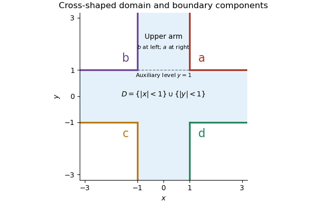
The cross-shaped domain, its four boundary values, and the auxiliary upper strip used for the limit at infinity
. Details. 
First justify finiteness of . A small open ball around lies outside the domain. By part (b), planar Brownian motion visits that ball almost surely in finite time. A continuous path from to that ball must meet first. Hence almost surely, and by continuity.
The harmonic function is smooth inside . The Itô formula, localized on relatively compact subdomains, makes a local martingale. Its boundary definition uses the continuous extension of . Since is bounded, this stopped process is a true martingale with uniform integrability: pass through the compact exhaustion using bounded convergence theorem. In particular .
Now almost surely as . The dominated convergence theorem, boundedness of , and its continuous boundary values give the bounded harmonic representation with almost sure Brownian exit:Almost sure exit and boundedness of the harmonic function are both used. The domain's unboundedness causes no loss of expectation here because the stopped function values are uniformly bounded.
Fix and start at with . Write the independent Brownian coordinates as and . LetOn the path has stayed in the upper strip and first exits the cross-shaped domain at its right or left side. The boundary value is or , respectively. Let if and if . The Brownian exit from an interval probabilities giveCouple all heights using the same two Brownian paths. By part (a), almost surely, and continuity makes finite. ThusLet . On the complement of this exceptional event, ; on the event itself, . The representation in part (c) therefore yieldsThis proves the harmonic limit along an infinite strip arm:Far up the arm, the bottom is reached with vanishing probability before the horizontal coordinate exits. The limit is consequently determined by the two side values alone.
A real Lévy process is a stochastic process with almost surely, independent increments, stationary increments, and stochastic continuity. The latter means in probability as . Its usual path convention is càdlàg: paths are right-continuous and have left limits. Equivalently one starts with the increment and continuity-in-probability conditions and then chooses the càdlàg version.
The Lévy characteristic exponent is specified here bySome conventions use instead, with . The sign convention must be fixed before computing the exponent. The zero process satisfies this definition; excluding it requires an additional nondegeneracy condition.
Both Poisson processes start at zero and have càdlàg paths. On disjoint time intervals their increments are independent, and independence of the two processes makes the difference increments independent as well. Their increment laws depend only on interval length, so has stationary increments. For a time interval of length , the probability that either Poisson process has a jump is . This proves stochastic continuity. Consequently the difference is a Lévy process, equivalently a continuous-time symmetric simple random walk with total jump rate one and jumps and each chosen with probability .
The characteristic function of a Poisson variable of mean is . Independence therefore givesThus, in the negative-exponent convention of part (a),In the positive-exponent convention the answer is . The Compound Poisson process has mean zero and variance , consistent with the expansion .
The printed uniqueness claim omits nondegeneracy of the limit. The zero process is a Lévy process, and every yields that limit. We first classify all possibilities under the stated assumptions, then identify the unique nonzero one.
For , part (b) givesfor each fixed . If , the characteristic functions tend to zero for every nonzero parameter and remain one at zero. This discontinuous function cannot be the characteristic function of a probability law. The characteristic-function convergence theorem therefore rules out even one-dimensional weak convergence of random variables at a positive time.
For joint convergence, take and write . Independent increments giveAt , this tends to . These are exactly the joint laws of standard Brownian motion: increments are independent centred normals with variances . The assumed limiting Lévy process thus has the Brownian law.
For , the same joint characteristic functions tend to one. Every limiting vector is zero. The càdlàg path convention then makes the limiting process identically zero almost surely: first intersect the zero-value events at rational times, then use right continuity. The complete scaling classification of a continuous-time symmetric simple random walk isIn particular, if a nonzero limiting Lévy process is intended, the unique exponent is , andThe finite-dimensional Brownian law, together with the Lévy càdlàg convention, determines the process law and its continuous version. No assertion of path-space convergence of the approximating walks is needed here.
Articles by others on the same topic
There are currently no matching articles.