For a twice continuously differentiable vector field in Cartesian coordinates, the curl and divergence arePut . Using the Levi-Civita symbol, the Kronecker delta contraction and the product rule,The last term vanishes because the divergence of a curl is zero: the symmetric mixed derivatives contract against an antisymmetric symbol. Thus the curl of a cross product identity becomes
For orthogonal coordinates with position vector , the scale factors of orthogonal coordinates and local unit vectors areOrthogonality gives , and right-handedness fixes . In cylindrical coordinates, , soThe radial vector points away from the axis; the azimuthal vector is tangent in the direction of increasing ; is the Cartesian positive direction. The azimuthal basis is undefined on the coordinate axis itself.
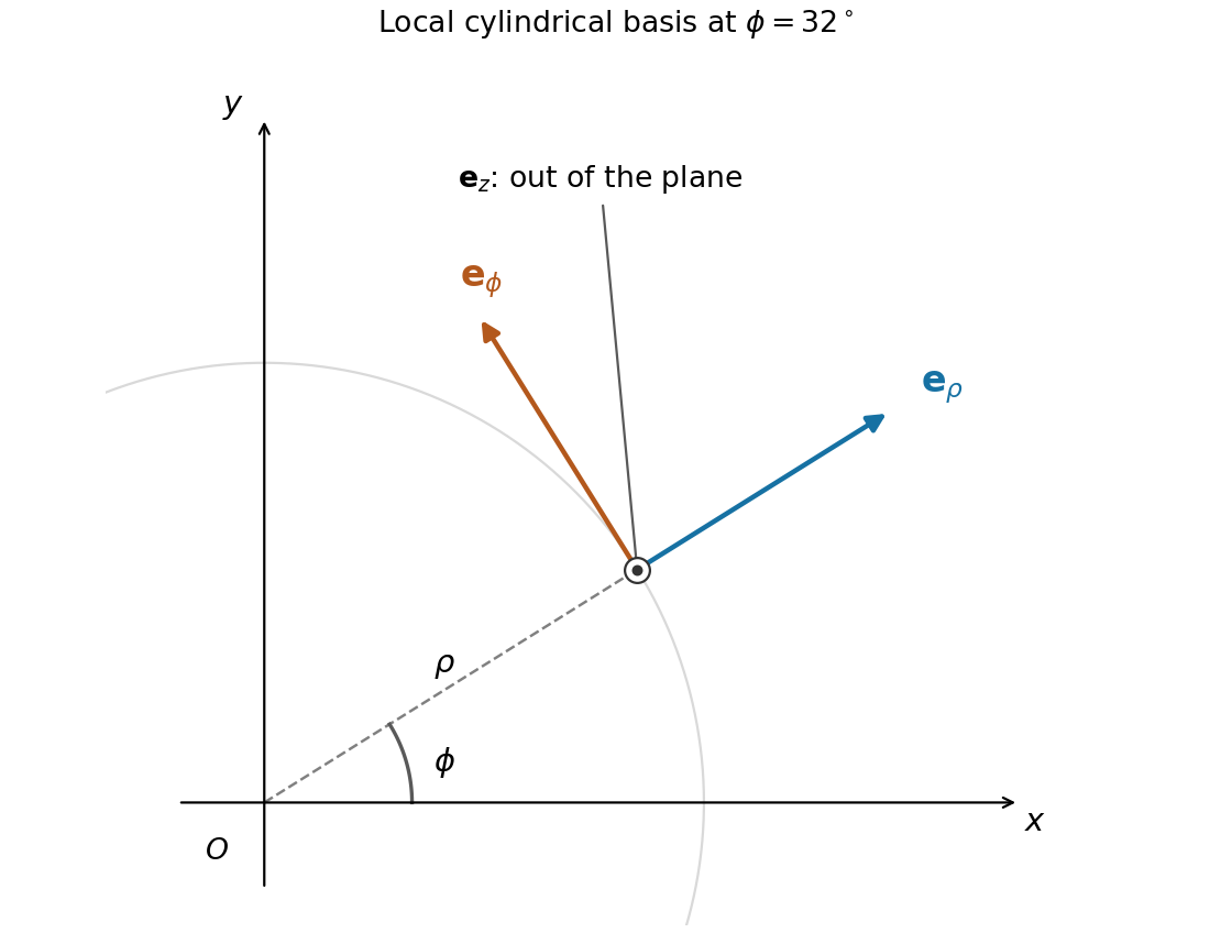
Cylindrical unit vectors relative to Cartesian axes, viewed from positive z
. Details. For the axial velocity profile, the cylindrical coordinates formula givesThe associated cross product isThis field has only a radial component depending on , so its curl is zero. Also . The identity above therefore yieldsIn fact both directional derivatives vanish: the first differentiates only in the azimuthal direction, and the second differentiates only in the direction. All physical vector fields extend smoothly through , despite the coordinate-basis singularity.
The substitution separates the uniform equilibrium from the decaying perturbation. Direct differentiation givesConsequently the reaction-diffusion equation reduces to the heat equation . Its data become
When the three constants coincide, the Dirichlet boundary conditions for are homogeneous. Separation of variables gives and , selecting the normal modes for . ThusTwo integrations by parts give , while the constant term uses . Therefore the Fourier sine series isFor , its first coefficient is nonzero. Multiplying by and retaining the slowest-decaying mode givesThe remainder estimate holds uniformly in for sufficiently large positive time. If , the fundamental vanishes and the next possible mode has decay rate , explaining the exclusion.
There is an initial endpoint compatibility issue unless : the given polynomial profile vanishes at the endpoints, whereas the boundary values equal . The series realizes the initial data in L2 space and pointwise in the open interval, imposing the prescribed boundary values for . For nonzero it cannot also be continuous at both initial endpoint corners.
Trying in the Cauchy-Euler equation givesso the homogeneous solution isContinuity with zero value at the singular endpoint excludes the second branch. Use the left and right adapted solutions , , whose Wronskian isThe Dirichlet Green kernel for an Euler operator with exponents one and minus four is thereforeIt vanishes at both endpoints, is continuous at , and has first-derivative jumpThus with ordinary source measure . For bounded forcing the Green function representation isThe apparent singular prefactor in the first term is canceled by the integral's decay at zero. The only regular homogeneous solution vanishing at is zero, so this solution is unique in the stated regular class.
For the piecewise source, split the integrals at . If , the needed integrals are and . If , only remains. Simplification yieldsAt the interface both expressions have value and derivative , so no unintended Dirac delta source appears. Their second derivatives have the allowed jump associated with the discontinuous forcing.
With the stated Fourier transform convention, the inverse Fourier transform and the deterministic autocorrelation of a square-integrable function areAssume initially sufficient decay and smoothness, for example a Schwartz function, to justify interchanging integrations and Fourier inversion. With , the cross-correlation identity isEvaluating directly and by its inverse transform at zero proves the Parseval identity:Approximation extends the identity to L2 space, as the Plancherel theorem.
For the compact cosine profile, the Fourier transform of a truncated cosine follows from :At the apparent singularities are removable, with value . The direct squared norm is . Hence Parseval identity and evenness givePutting makes the left side times the requested integral. ThereforeAt the integrand's continuous extension is , so no principal-value prescription is required.
A square matrix is invertible precisely when its determinant is nonzero. Equivalent conditions are full rank, a trivial kernel, and zero not being an eigenvalue.
For a lower triangular matrix, the first row has only the possibly nonzero entry . A Laplace expansion along that row gives , where the remaining principal submatrix is again lower triangular. Induction from the one-by-one case yieldsThis proof includes singular triangular matrices; it makes no division by diagonal entries.
For the diagonal example, put . Its determinant is , and invertibility requires . Write the complex number as with . A nonzero purely imaginary determinant requires . ThusEquivalently ; the angle is understood modulo .
For skew-Hermitian matrices, reversing products under the conjugate transpose gives . ConsequentlyThe latter condition is vanishing of the anticommutator. A universal choice for the last request isIndeed , so the commutator of two skew-Hermitian matrices is skew-Hermitian.
Over the chosen scalar field, an -by- matrix is diagonalizable if and only if it has linearly independent eigenvectors. Repeated eigenvalues are allowed provided all eigenspaces together supply a basis.
For the given matrix, the characteristic polynomial is . One may chooseTaking these as columns gives the change of basisThis is not a rotation matrix. The PDF's terminology cannot hold literally: is real and nonsymmetric, whereas a real matrix orthogonally similar to a real diagonal matrix is symmetric. Also , so scaling these eigenvectors cannot make an orthonormal rotation basis. A general invertible similarity is the valid construction.
Let . Inserting between successive factors gives , and henceTo write , match its action on the two eigenspaces:Solving gives the matrix powers for a diagonalizable matrix with two eigenvaluesThe cases recover , respectively. Equivalently the spectral projections of a diagonalizable matrix are and , and the power multiplies them by and .
The Cauchy-Riemann equations are and . A holomorphic function is smooth, so equality of mixed partial derivatives givesThus its real and imaginary parts are harmonic functions.
An entire function is holomorphic at every finite point of the complex plane. The globally convergent power series for the exponential implies that and are entire. Their difference therefore givesat every complex , proving that the hyperbolic sine is entire. For powers, the base case has derivative one everywhere. If is entire with derivative , the product rule gives everywhere. Induction proves that every positive integer power is entire.
A function has a pole of order at when it is holomorphic in a punctured neighbourhood and extends holomorphically to with . An isolated essential singularity is neither a removable singularity nor a pole; equivalently its Laurent series has infinitely many nonzero negative-power terms. In particularhas an essential singularity at zero.
For , the Laurent series about infinity isTo classify the point correctly, use . Then , and is holomorphic with value one at zero. ThereforeThe pole at infinity is compatible with an essential singularity at the finite point zero. Negative powers of are regular powers of the local coordinate near infinity, so they do not make that point essential.
Write a second-order linear ordinary differential equation in monic form . At a finite point , an ordinary point has analytic . A singular point is a regular singular point if and extend analytically there. A singular point failing this condition is an irregular singular point. The point at infinity is classified by the reciprocal coordinate .
For the Laguerre differential equation, and . Thus and are analytic at zero, while itself is singular: zero is regular singular. Put . Since and , the transformed equation isHere is not analytic at zero, so infinity is an irregular singular point, for every real .
For the Frobenius solution, the lowest power has coefficient . Hence the indicial equation is , and equating the remaining powers givesWith the repeated root , the Frobenius series for the Laguerre differential equation obeysIf the series does not terminate, its consecutive term ratio is asymptotic to , so the ratio test gives infinite radius of convergence. It is an entire function, even though the differential equation has a singular coefficient at zero. The repeated indicial root yields only one analytic Frobenius branch; an independent solution generally has a logarithmic term there.
For , the factor stops the recurrence at degree . With its coefficients are , giving the Laguerre polynomialsThe same termination argument includes , as required for despite the earlier reference to positive integers.
For endpoint-preserving variations of a functional, the Euler-Lagrange equation isAlong an extremal, the chain rule gives . Thus when has no explicit dependence, the Beltrami identity isFor a positive speed profile, the elapsed-time integrand in Fermat principle is . Its first integral givesIntegrating each monotone-height branch yieldsReal branches require . Turning points are joined in the original graph , even though the inverse derivative is singular there.
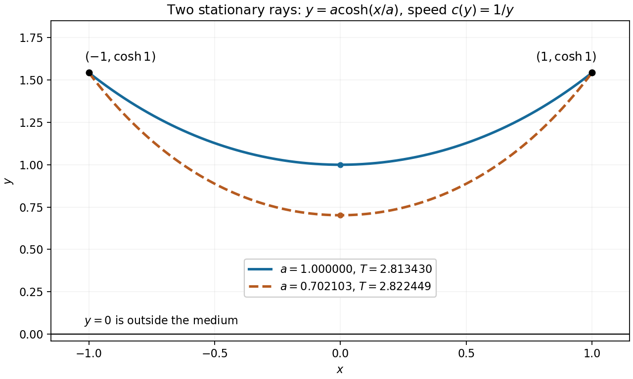
For the inverse-height speed profile, this becomes , with . Integration gives , so the light rays are catenariesEqual endpoint heights at opposite values force , since the real hyperbolic cosine is even and strictly increases with the absolute value of its argument. The remaining endpoint condition is . One exact solution is , givingHere and account for the squared hyperbolic cosine in the time integral.
The stated endpoints also allow a second stationary ray. Set . The function decreases and then increases: its derivative has the sign of , whose derivative is . Its unique minimum occurs where , at . Since the known root lies below this minimum's location, there is exactly one further root, . Thus the two stationary catenary rays in an inverse-height speed profile also includeNo extra condition in the question selects uniquely between these rays. The minimum height is a minimum along the chosen ray, not a global travel-time assertion. Indeed, competitors descending vertically to height , crossing horizontally, and rising again have time . As this tends to , below both stationary times. Their corners can be smoothed, so Fermat principle here must be understood as stationarity rather than unrestricted global minimization.


Use a Lagrange multiplier for the norm constraint. For real variations with , integration by parts givesThus stationarity is equivalent to the Sturm-Liouville problemMultiplying by and integrating shows , so the constrained stationary values are the eigenvalues, and the normalized stationary functions are their eigenfunctions. Conversely the eigenvalue equation makes the constrained first variation vanish. The self-adjoint operator has weight one.
For , zero and negative eigenvalues yield no nonzero solution with both Dirichlet boundary conditions. Positive eigenvalues have solutions after the left condition, and the right condition gives , . Hence the lowest eigenpair iswhere the amplitude follows from .
The Rayleigh-Ritz variational principle bounds the full lowest eigenvalue by . Its derivative contribution is one. For the linear potential, reflection about givesThus the sine trial bound for a linear potential on an interval isFor the bound is strict, since is not a constant multiple of . Also by the Poincaré inequality and the nonnegative potential. Equality in the upper bound holds at .
Articles by others on the same topic
There are currently no matching articles.