The dynamical method. In Lagrangian mechanics, choose independent generalized coordinates consistent with the constraints, form the Lagrangian , and solve the Euler-Lagrange equations,This form applies to a Newtonian system with ideal constraints, so constraint forces do no allowed virtual work, and with the remaining forces derivable from the stated potential. Smooth holonomic constraints can be built into the coordinates. Additional nonconservative generalized forces would appear on the right. Prescribed shaft rotation is a driven constraint; its constant is a parameter, not a conserved angular momentum.
Energy of the two balls. The diagram labels each ball , so their combined mass is . It also shows between an arm and the downward vertical, rather than the full angle between the arms. Each ball has horizontal radius , vertical coordinate , and squared speed . ThusandThe massless connecting rods and sliding collar enforce the geometry but contribute no energy.
Effective potential. Define . At fixed ,This effective potential determines the reduced dynamics. Its conserved effective energy is not the full lab-frame mechanical energy: the shaft drive can exchange work and angular momentum with the balls.
The change of stability. Near ,For , the downward state is a minimum. At , its quadratic stiffness vanishes but the quartic coefficient is . Above that speed, the downward state becomes a maximum and stable nonzero openings appear. This is the gravity-restored centrifugal governor bifurcation.
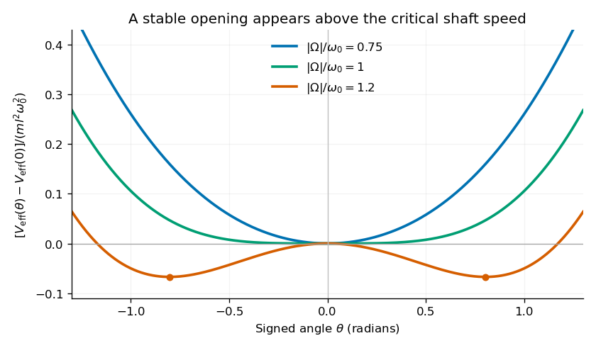
Original calculated effective potentials below, at and above the critical shaft speed; signed angles display the symmetric mathematical extension of the opening coordinate
. Details. 
The physical opening is nonnegative; the two minima in the signed extension represent opposite transverse displacements. The stable opening increases continuously from zero toward a right angle as grows. The apparatus is frictionless in the model, so a displaced system oscillates rather than automatically settling at the equilibrium shown by the minima.
Equilibria. Differentiation givesHence the downward equilibrium is , and the open equilibria satisfyThe signed extension includes the negative of this angle. Formally is also stationary, but it is an unstable inverted configuration and lies outside the usual opening range of the mechanism.
Small oscillations. Write . The linear equation is , whereAt the downward state and at a nonzero open state, respectively,These are angular frequencies in ; ordinary frequencies are . Negative indicates exponential instability rather than an oscillation. At , . At the critical speed, the linear frequency is zero and the positive quartic potential gives amplitude-dependent nonlinear restoring motion.
Classification of attractive inverse-square orbits. Write the potential energy as , with and zero at infinity. For nonzero angular momentum , the Kepler orbit is a conic,Negative total orbital energy gives an elliptic orbit, . Its special case is the circular Kepler orbit, at the minimum energy permitted for that , . Zero energy gives a parabolic Kepler orbit, , and positive energy a hyperbolic Kepler orbit, . For , the motion is radial: these are degenerate limiting trajectories and may strike the centre or the finite planetary surface.
The scattering geometry. The impact parameter is the perpendicular offset of the undeflected incoming asymptote from the centre, not the actual periapsis radius . Gravity bends the incoming path toward the planet.
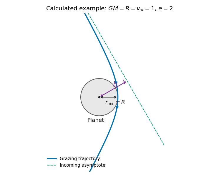
Original calculated grazing hyperbola with its incoming asymptote, impact parameter and periapsis; the planet and trajectory use a dimensionless illustrative choice
. Details. 
The grazing threshold. At infinity, conservation of energy and angular momentum give and . At closest approach the radial speed is zero, so the velocity is tangential andEliminating givesThis increases monotonically with . Setting gives the grazing impact parameter in gravitational focusing,Here is the surface escape speed. The expression has units of length. Equality is the tangency limit; a strictly noncolliding trajectory requires . At high speed, , while at low speed . Thus gravitational focusing enlarges the collision cross-section to .
Deflection angle. For this hyperbola,The asymptotes occur at . The change of velocity direction is , giving . Hence the gravitational scattering angle satisfiesFor the grazing trajectory this isIt is the attractive counterpart of the Rutherford impact-parameter relation; the sign of the transverse bending changes, but the positive deflection magnitude has this same form.
Range of angles. Along the grazing family, varying givesThe limits are as and as . Neither endpoint is reached at finite positive speed. The low-speed limiting orbit still has a finite periapsis, but an increasingly distant incoming asymptote.
Modes, stability and symmetry. A normal mode of the linearized system has a fixed displacement pattern multiplied by one temporal oscillation. For independent generalized coordinates, a conservative small-disturbance system hasWhen the mass matrix is positive definite and the stiffness is a symmetric matrix, the generalized eigenvalue problem for small oscillations has independent mode directions, counting degeneracy. Positive gives stable oscillation, negative an exponentially growing and decaying pair, and zero a neutral direction whose nonlinear stability needs further analysis. An arbitrary linear motion is a superposition of these modes.
If a symmetry preserves both kinetic and potential energies, it maps modes to modes of the same frequency. Mode patterns can be classified by that symmetry, for example reflection-even and reflection-odd patterns. Degenerate eigenspaces admit different bases, so a mode shape need not be uniquely selected inside such a subspace.
Two pendulums free to swing in any direction. Let be the small horizontal displacement along the line joining the supports and the perpendicular horizontal displacement. Put and . To quadratic order,The spring is unstretched at equilibrium. Its first-order length change is only ; a transverse difference changes its length at second order and produces no quadratic transverse restoring energy. Consequently the four modes areThis is the transverse degeneracy of unstretched spring-coupled pendulums: has a three-dimensional eigenspace. Independent transverse motions form an equally valid basis for two of those directions. A pre-tensioned spring would change the transverse result.
The open three-pendulum chain. Restrict motion to the vertical plane containing the supports, with horizontal coordinates . There are springs between neighbours and no wall springs. The equations areThe spring matrix has eigenvalues , with respective eigenvectors , and . The normal modes of three freely ended coupled pendulums are thereforeThe lowest mode stretches neither spring. In the middle mode the outer masses oppose each other and the central mass is stationary. The highest mode has the central mass moving oppositely with twice the outer amplitude. Reflection about the middle support makes the first and last patterns even and the middle pattern odd.
An even ring. For a large ring, use tangential displacement and periodic indexing . The locally straight nearest-neighbour equations areCyclic translation symmetry selects Fourier modes , with . HenceFor even , the lowest pattern has equal tangential displacements, while the highest alternates signs around the ring. Thus
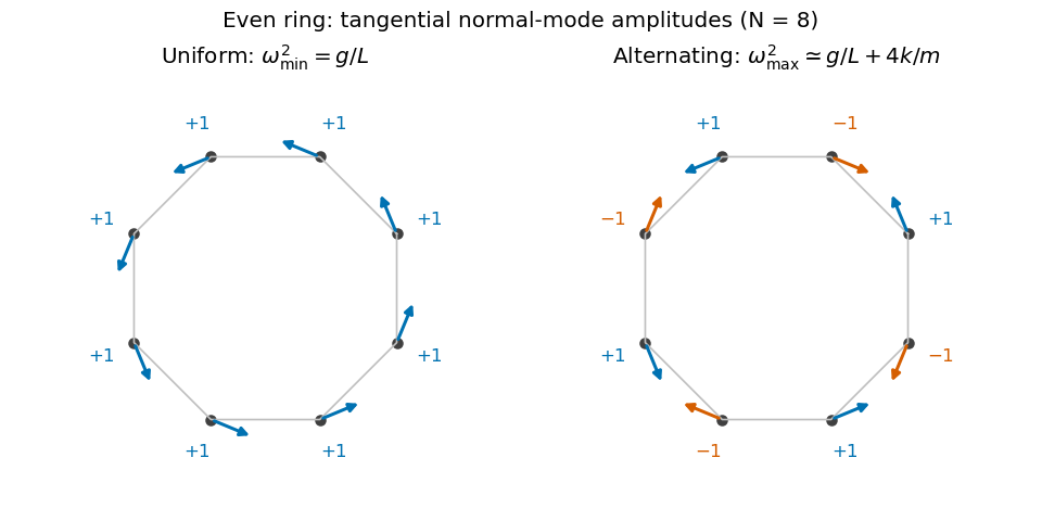
Original amplitude sketches for the lowest and highest modes of an even pendulum ring; arrows denote tangential displacements, not static positions
. Details. 
These are the even and odd pendulum-ring modes. For exact finite regular-polygon geometry with straight chord springs, the first-order spring extension includes a factor , so its squared contribution is multiplied by . That correction tends to one in the requested large- limit.
An odd ring. Perfect alternation cannot close after an odd number of steps. The two highest wave indices are instead and . They give a degenerate pair, represented by real sine and cosine standing patterns, withThe maximum is slightly below the even-ring limiting value, and the sign pattern must contain a gradual phase mismatch rather than exact alternation. The uniform lowest mode is unchanged, and there are still independent tangential mode directions.
Flow visualization and the idealization. A streamline is everywhere tangent to the instantaneous velocity field at one fixed time. A streakline is the locus, at one observation time, of particles that previously passed through a specified injection point. A marked particle's own trajectory is a pathline. These coincide geometrically in steady flow, but need not do so in an unsteady draining flow.
The intended ideal liquid is approximately incompressible and inviscid: viscosity and associated shear stresses are negligible on the scales and times being considered, the Mach number is small, and the density is effectively constant. This does not require zero vorticity; the initially rotating state is already a counterexample. It also does not justify ignoring viscosity in an arbitrarily thin boundary layer or at a real drain.
Spiralling flow and angular momentum. In an axisymmetric inviscid flow, pressure and gravity exert no torque about the vertical axis. A parcel therefore conserves axial specific angular momentum,The late, shallow remnant in the intended draining picture is supplied by parcels initially near the outer rim, so . The slow-drain angular-momentum amplification then givesThe assumption about the parcels' origin is necessary: torque conservation by itself does not assign to every parcel at every time.
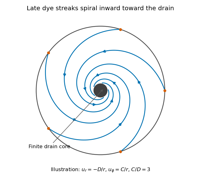
Original quasisteady illustration of inward-spiralling dye streaks outside a finite drain core; the azimuthal speed increases as the radius decreases
. Details. 
A continuous dye feed near the outer free surface produces inward spirals that wind increasingly rapidly near the drain. The figure uses a late quasisteady model, and with positive constants , giving . Its streaklines and streamlines approximately coincide over an observation interval short compared with the overall draining time. Strictly, individually marked particles at the initial surface trace pathlines, not a continuously injected streakline.
The free-surface depression. Let be the surface. Slow radial draining makes radial inertial corrections small compared with the azimuthal centripetal acceleration. The radial Euler equation and vertical hydrostatic equilibrium giveThus , with . Integrating from to the rim givesFor this becomesThe surface rises outward because the inward pressure gradient force must sustain the circular motion. The dimensions are metres, and the profile is not valid inside the finite drain or vortex core.
The terrestrial estimate. Use the vertical component of Earth's rotation as the ideal initial angular speed, . At Cambridge, taking and , this gives . Hence, for , and ,Taking the whole terrestrial angular speed rather than its local vertical projection would give about . The Cambridge estimate uses the projection appropriate to the vertical vortex. This very small head assumes terrestrial rotation supplies the only initial swirl; imposed residual rotation would change it quadratically.
Curl of the azimuthal velocity. For axisymmetric with no vertical dependence, the rotational part of the vorticity is vertical:The ideal quasisteady radial sink has no curl outside its core. The source's symbol denotes this vertical vorticity component, not the fluid's angular velocity. In general its magnitude is the absolute value of the bracket.
The two limiting states. For initial uniform rotation, , whereas the late approximation has . ThereforeThe late flow can have large angular velocity and nonzero circulation while being locally irrotational. The drain core is excluded from the domain of the velocity field.
What is actually conserved. Inviscid does not mean that each parcel's vorticity magnitude is fixed in three dimensions. For an incompressible barotropic liquid with conservative body forces, the vorticity equation isVertical compression of a material column changes its vorticity through vortex stretching, even while its volume is conserved by horizontal expansion. In the columnar shallow-layer limit, vorticity dilution in a shallow draining layer givesThus a remnant much shallower than its original column can have much smaller vertical vorticity. At finite depth there is generally a residual value; the exactly irrotational late profile is a leading limiting approximation, not an exact parcelwise conversion of nonzero vorticity to zero in finite time.
Kelvin's circulation theorem conserves circulation around a material loop, not around a fixed spatial circle. A loop whose original radius is near has circulation about , consistent with the late field. Fluid also leaves through the drain, so the remaining tank contents are not a fixed material system. If the calculation is expressed explicitly in the Earth-fixed rotating frame, the corresponding shallow-water potential vorticity is , with ; the conserved quantity involves absolute vorticity.
Articles by others on the same topic
There are currently no matching articles.