For two circular Kepler orbits about the same body, Kepler's third law gives . The reference radius is measured from Earth's centre:A geostationary orbit is prograde and equatorial, with one sidereal day as its orbital period. Using and the supplied ,Using instead changes this estimate by less than one per cent. This is the orbital radius, not the altitude; the corresponding altitude is about .
There is a numerical inconsistency in the source data. The quoted reference orbit implies , appreciably below the measured terrestrial value, about . Using the latter instead gives the familiar geostationary orbit radius . The boxed estimate consistently uses the period actually printed in the question.
The radial force is . A nontrivial circular orbit therefore requires , so that the force is inward. Balancing its magnitude against the required centripetal acceleration givesThusThis is the circular-orbit energy ratio in a power-law potential, for , with . It uses the zero of potential energy specified by ; adding a constant would change the ratio without changing the motion. For , the force is outward and no such free circular orbit exists.
For linear elasticity of an isotropic material, the isotropic elastic modulus relation givesThe printed Young's modulus is , and the printed Poisson's ratio is . Formal substitution givesWith compressive pressure positive, the linear volume response is . Thus a thirty per cent reduction formally requiresHere . The negative pressure is a formal tensile load, not the requested positive isotropic compression.
The original PDF really prints . It is incompatible with a stable ordinary isotropic elastic solid: positive bulk modulus and shear modulus require . Consequently there is no physically admissible positive-pressure answer with the stated constants. If was intended, the corresponding linear estimates would instead beThat is an explicit alternative, not a correction established by the source. A thirty per cent volume strain is also outside a controlled small-strain approximation; accurate rubber behaviour at that deformation needs a finite-strain constitutive law. The initial volume cancels because the specified change is a fractional one.
Closest approach. In the heavy-target approximation, a head-on alpha particle of charge converts its initial kinetic energy to repulsive Coulomb potential energy at its turning point. The nuclear radius bound from a Coulomb turning point is thereforeThus the point-projectile interpretation of the radius bound isIt is an upper limit from Coulomb scattering, not a measurement of the actual nuclear radius. If “size” denotes diameter, the associated bound is twice this value. Including nuclear recoil, , increases the closest separation by about two per cent to .
Count-rate estimate and normalization. The graph has approximate slope . It therefore supplies the empirical log-log plot relation . Calibrating its normalization with the lead observation givesThe Rutherford differential cross-section at fixed beam energy and scattering angle instead has a dependence per target nucleus. More generally, the target normalization in Rutherford scattering rates iswhere is the target nuclei per unit area. If the foils have equal , the theoretical estimate is , or about particles per minute, close to the graphical estimate at its rough level. Equal foil mass per area would instead give per minute because .
The source does not specify that target normalization. Thus per minute is the estimate from its supplied graph; an exact rate prediction from Rutherford theory alone is underdetermined without comparable foil areal densities. The empirical slope and an exact equal- law should not be presented as identical assumptions.
For a reversible adiabatic process, an ideal gas obeys . A monatomic gas has heat capacity ratio . Taking the stated expansion factor to mean ,This assumes the usual quasistatic isentropic process. Heat insulation alone does not determine the final temperature: an ideal-gas free expansion is also adiabatic but leaves the temperature unchanged. The numerical answer uses nine times the original volume, the conventional intended meaning of the source's “nine times larger”.
The original PDF places this complete question before B6 without a visible question number. It is included here under a descriptive heading.
Why images work. In the method of images, place fictitious image charges outside the region where the physical electric field is required. Choose them so that the combined electric potential satisfies the conductor boundary conditions. The Uniqueness of the Dirichlet problem then proves that this construction gives the physical exterior field. The images do not describe the actual surface-charge locations.
Two examples are a charge above a grounded conducting plane, represented by at the mirror point, and the image charge for a grounded conducting sphere used below. In each case the image lies inside the excluded conductor and makes its surface an equipotential of the required value.
Potential of the two charges. By the law of cosines, the distances from the observation point to charges at are . The superposition principle and Coulomb's law therefore give
The grounded sphere. Set and require at every polar angle. Matching the coefficients of and the constant terms givesThe useful noncoincident solution isIndeed on the sphere, so the two potential terms cancel there. A Gaussian surface enclosing the sphere but not the external charge measures the total image charge in the exterior representation. Thus the physical induced net charge is
An isolated neutral sphere. The grounded image would give nonzero net charge. Add a central image to cancel it. A central image changes the surface potential by a constant, preserving the equipotential condition, whereas an arbitrary off-centre image would generally spoil it. The image charges for a neutral conducting sphere giveThe potential is measured relative to zero at infinity for each finite .
Fixed applied field and dipole moment. For positive on the positive axis, the applied central field is . The central image contributes no electric dipole moment, soIts units are coulomb metres. Keeping fixed makes constant, so this induced moment is independent of the distance.
The distant-charge limit. As with fixed, the applied field becomes uniform over any fixed neighbourhood of the sphere. The neutral pair of opposite images approaches a point dipole of the finite moment above. The external potential contains a growing spatial constant , so the infinity-referenced conductor potential does not have a finite limit. Subtracting this irrelevant constant gives the usual induced charge on a conducting sphere in a uniform electric field; the exterior potential becomesThis has zero potential on the sphere, but a uniform applied field cannot simultaneously have its potential vanish at spatial infinity.
Induction and its sign. The Maxwell-Faraday equation is . For a fixed loop, Stokes theorem givesThis is Faraday's law of induction. The orientation of the surface normal and positive circulation are linked by the right-hand rule. The minus sign is Lenz's law: the induced current's linked flux opposes the imposed flux change, rather than reinforcing it.
The inductive current. Let the loop normal make angle with the applied field, with positive current defined by that normal. The external magnetic flux is . With negligible electrical resistance, the circuit equation is , so total linked flux is constant. For zero initial trapped flux,The printed result needs this initial-flux assumption; in general an additional constant current is allowed. The units are amperes because a weber divided by a henry is an ampere.
Current and forces at one instant. Take along and , so relative to the chosen normal. The loop magnetic dipole moment therefore has a component opposite the applied field. Each wire element experiences Lorentz force . Opposite sides have equal and opposite forces, giving zero net force in the uniform field but a nonzero couple.
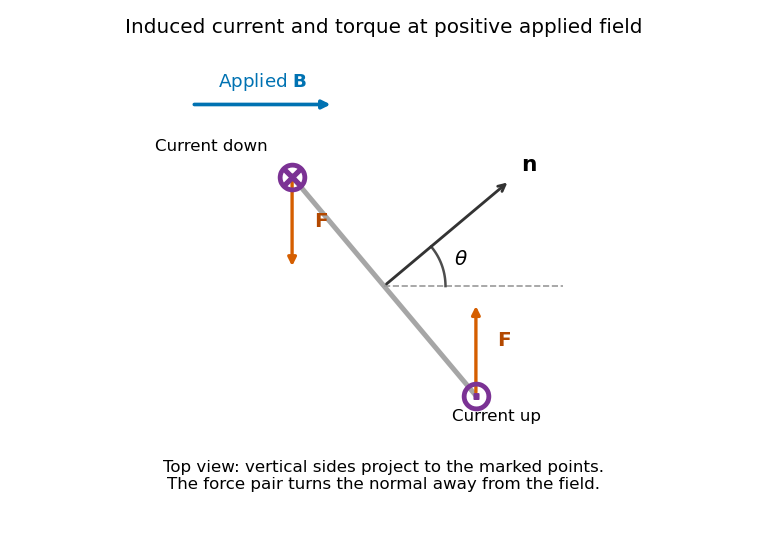
Original top view of the loop's vertical sides at positive applied field; dots and crosses show vertical current, and the force pair increases the angle between normal and field
. Details. The horizontal top and bottom wire segments also experience equal and opposite vertical forces. They cancel without adding torque about the vertical rotation axis; the displayed force pair supplies that torque.
Average torque. Since , its generalized component for increasing is . Substitution givesand, using ,The orientation torque on a flux-conserving loop drives its normal away from the field for the stated initial angle. Its magnitude has units joules, or newton metres.
Free motion with large inertia. Write for the mechanical moment of inertia. If its orientation changes little during each field cycle, the slow equation is , with effective potentialThe stable orientation is , where the loop plane contains the applied field. Released from rest between and , the loop accelerates toward that orientation, overshoots and librates around it. In the leading averaged, undamped model its turning angles are and . It does not settle without a dissipative mechanism. For small librations the squared angular frequency is .
Negligible inductance and finite resistance. Now the current is proportional to the induced electromotive force, not to the flux. Including slow rotation,The rotational damping of a resistive loop in an oscillating field follows fromAt fixed orientation, the first term alternates at and has zero mean. The loop can therefore rock slightly, but there is no leading mean aligning torque like that in the inductive case. Slow rotation giveswhich opposes motion and produces Joule heating. Initial-phase transients can initiate motion, and the instantaneous torque is not zero. This description retains the large-inertia, slow-motion approximation; it does not assert an exact stationary solution at every starting angle.
The integral field equation. The Ampere-Maxwell law is . Apply Stokes theorem to any fixed oriented surface bounded by the chosen contour:The added displacement current is required for compatibility with electric charge conservation. Taking a divergence and using gives .
Field geometry. Choose the upper plate positive and let increase upward. In the long-plate, slow-discharge approximation, . Conventional wire current runs downward from the positive plate. The magnetic field intensity circulates clockwise as viewed from above. The Poynting vector points radially toward the resistive wire.
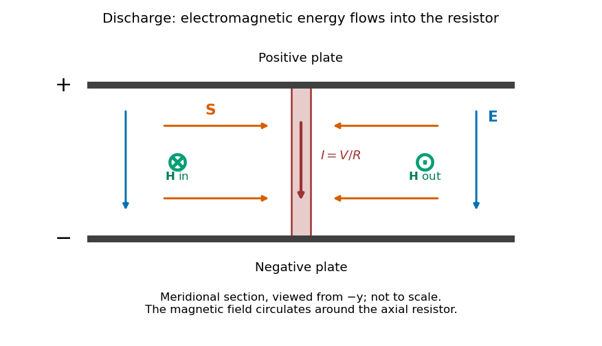
Original meridional section of the discharging capacitor; electric field and wire current point down, magnetic field circles the wire, and electromagnetic energy flows inward
. Details. Wire and displacement currents. The capacitance and discharge law areBecause decreases, points upward, opposing the downward wire current. Through a disk of radius between the plates its magnitude isThe effective downward current enclosed by the circular contour is therefore . The Ampere-Maxwell law givesThis is the magnitude; with the stated coordinates, . The factor expresses cancellation between conduction and displacement currents. The approximation requires distances outside the thin wire and away from detailed electrode-edge fields.
Energy flux and power. Since ,Its units are watts per square metre. Integrating over the cylinder's side area , the signed outward power is negative:There is no leading axial flux through the cylinder's ends in this ideal field geometry.
Where the energy goes. The Poynting flux in a centrally discharged parallel-plate capacitor carries field energy through the dielectric space into the resistor, where it becomes Joule heating at rate . Inside radius the stored electric energy isHenceThe resistor receives the inward flux from outside that cylinder plus the field energy released inside it. As approaches the wire radius, essentially all its power arrives as radial electromagnetic flux. Over the whole capacitor, . The Poynting theorem thus accounts for the complete discharge without treating energy as transported only along the conducting wire. High resistance makes the quasistatic electric-field approximation and neglect of changing magnetic energy consistent.
Two interface effects. For , Snell's law gives . If , no propagating transmitted ray exists: there is total internal reflection, with an evanescent wave on the far side. An optical fibre uses this to guide light.
For ordinary isotropic nonmagnetic media, is the Brewster angle. The reflected p-polarized component, whose electric field lies in the incidence plane, vanishes; the reflected s-polarized component generally remains. Reflection polarizers and polarized glare reduction exploit this selectivity.
The plasma response. Neglect collisions, thermal-pressure corrections and background magnetic field. Let the wave vary as . An electron displacement obeysIts dipole moment is , so the electron electric polarization is . Ions of charge give a further contribution , smaller by . Thus heavy ions move negligibly at these electron-wave frequencies. Using gives the cold collisionless plasma dielectric response,For this model , so and for the transverse electromagnetic wave.
The vertical cutoff and density. Below the plasma frequency, the squared refractive index is negative: the wave is an evanescent wave instead of propagating through a layer hundreds of kilometres thick. The observed cutoff therefore identifies , with . ConsequentlyThis uses , and . The density is also .
The transmission elevation. At , the ionosphere has refractive indexIf is elevation above horizontal, incidence at the layer is . Avoiding total internal reflection requires . The limiting elevation is thereforeStrictly, it must point above this limiting angle to carry upward power through the finite layer: at equality the transmitted wave is grazing. With a suitable satellite position, the stated orbital altitude imposes no additional angular constraint in this flat-layer approximation.
Polarization-selective ground reflection. The ray's incidence plane is vertical. Horizontal electric polarization is s polarization; the other transverse polarization lies in the vertical incidence plane and is p polarization. Reflection of s but not p identifies the Brewster angle, not total internal reflection, which would reflect both in this lossless isotropic model. ThusFor a reflecting height , the horizontal range consists of two equal legs. The Brewster reflection from an ionospheric interface givesAt this angle is below the critical incidence angle, so a transmitted ray also exists; the detected horizontal component is an ordinary partial reflection. The s-polarized reflected power fraction is approximately , whereas the ideal p-polarized reflected fraction is zero. These results use the question's sharp planar interface model and exclude upper-interface reflections.
The dynamical method. In Lagrangian mechanics, choose independent generalized coordinates consistent with the constraints, form the Lagrangian , and solve the Euler-Lagrange equations,This form applies to a Newtonian system with ideal constraints, so constraint forces do no allowed virtual work, and with the remaining forces derivable from the stated potential. Smooth holonomic constraints can be built into the coordinates. Additional nonconservative generalized forces would appear on the right. Prescribed shaft rotation is a driven constraint; its constant is a parameter, not a conserved angular momentum.
Energy of the two balls. The diagram labels each ball , so their combined mass is . It also shows between an arm and the downward vertical, rather than the full angle between the arms. Each ball has horizontal radius , vertical coordinate , and squared speed . ThusandThe massless connecting rods and sliding collar enforce the geometry but contribute no energy.
Effective potential. Define . At fixed ,This effective potential determines the reduced dynamics. Its conserved effective energy is not the full lab-frame mechanical energy: the shaft drive can exchange work and angular momentum with the balls.
The change of stability. Near ,For , the downward state is a minimum. At , its quadratic stiffness vanishes but the quartic coefficient is . Above that speed, the downward state becomes a maximum and stable nonzero openings appear. This is the gravity-restored centrifugal governor bifurcation.
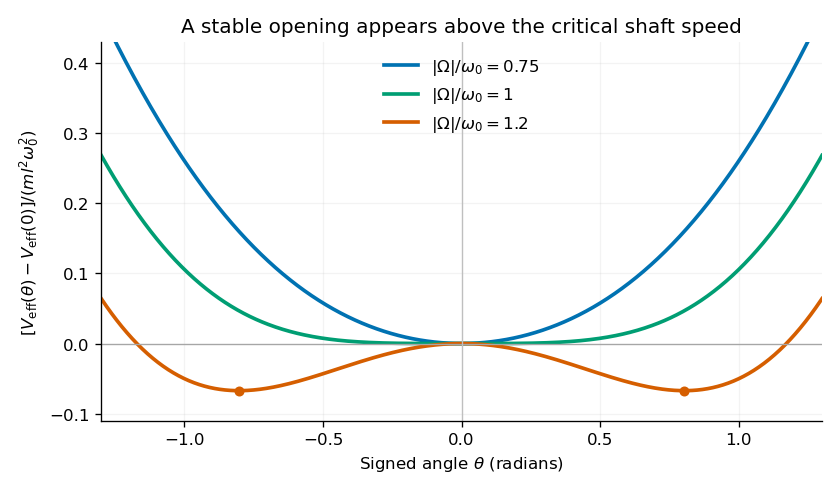
Original calculated effective potentials below, at and above the critical shaft speed; signed angles display the symmetric mathematical extension of the opening coordinate
. Details. The physical opening is nonnegative; the two minima in the signed extension represent opposite transverse displacements. The stable opening increases continuously from zero toward a right angle as grows. The apparatus is frictionless in the model, so a displaced system oscillates rather than automatically settling at the equilibrium shown by the minima.
Equilibria. Differentiation givesHence the downward equilibrium is , and the open equilibria satisfyThe signed extension includes the negative of this angle. Formally is also stationary, but it is an unstable inverted configuration and lies outside the usual opening range of the mechanism.
Small oscillations. Write . The linear equation is , whereAt the downward state and at a nonzero open state, respectively,These are angular frequencies in ; ordinary frequencies are . Negative indicates exponential instability rather than an oscillation. At , . At the critical speed, the linear frequency is zero and the positive quartic potential gives amplitude-dependent nonlinear restoring motion.
Classification of attractive inverse-square orbits. Write the potential energy as , with and zero at infinity. For nonzero angular momentum , the Kepler orbit is a conic,Negative total orbital energy gives an elliptic orbit, . Its special case is the circular Kepler orbit, at the minimum energy permitted for that , . Zero energy gives a parabolic Kepler orbit, , and positive energy a hyperbolic Kepler orbit, . For , the motion is radial: these are degenerate limiting trajectories and may strike the centre or the finite planetary surface.
The scattering geometry. The impact parameter is the perpendicular offset of the undeflected incoming asymptote from the centre, not the actual periapsis radius . Gravity bends the incoming path toward the planet.
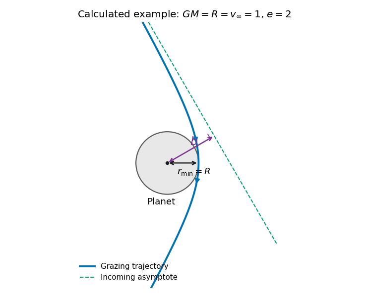
Original calculated grazing hyperbola with its incoming asymptote, impact parameter and periapsis; the planet and trajectory use a dimensionless illustrative choice
. Details. The grazing threshold. At infinity, conservation of energy and angular momentum give and . At closest approach the radial speed is zero, so the velocity is tangential andEliminating givesThis increases monotonically with . Setting gives the grazing impact parameter in gravitational focusing,Here is the surface escape speed. The expression has units of length. Equality is the tangency limit; a strictly noncolliding trajectory requires . At high speed, , while at low speed . Thus gravitational focusing enlarges the collision cross-section to .
Deflection angle. For this hyperbola,The asymptotes occur at . The change of velocity direction is , giving . Hence the gravitational scattering angle satisfiesFor the grazing trajectory this isIt is the attractive counterpart of the Rutherford impact-parameter relation; the sign of the transverse bending changes, but the positive deflection magnitude has this same form.
Range of angles. Along the grazing family, varying givesThe limits are as and as . Neither endpoint is reached at finite positive speed. The low-speed limiting orbit still has a finite periapsis, but an increasingly distant incoming asymptote.
Modes, stability and symmetry. A normal mode of the linearized system has a fixed displacement pattern multiplied by one temporal oscillation. For independent generalized coordinates, a conservative small-disturbance system hasWhen the mass matrix is positive definite and the stiffness is a symmetric matrix, the generalized eigenvalue problem for small oscillations has independent mode directions, counting degeneracy. Positive gives stable oscillation, negative an exponentially growing and decaying pair, and zero a neutral direction whose nonlinear stability needs further analysis. An arbitrary linear motion is a superposition of these modes.
If a symmetry preserves both kinetic and potential energies, it maps modes to modes of the same frequency. Mode patterns can be classified by that symmetry, for example reflection-even and reflection-odd patterns. Degenerate eigenspaces admit different bases, so a mode shape need not be uniquely selected inside such a subspace.
Two pendulums free to swing in any direction. Let be the small horizontal displacement along the line joining the supports and the perpendicular horizontal displacement. Put and . To quadratic order,The spring is unstretched at equilibrium. Its first-order length change is only ; a transverse difference changes its length at second order and produces no quadratic transverse restoring energy. Consequently the four modes areThis is the transverse degeneracy of unstretched spring-coupled pendulums: has a three-dimensional eigenspace. Independent transverse motions form an equally valid basis for two of those directions. A pre-tensioned spring would change the transverse result.
The open three-pendulum chain. Restrict motion to the vertical plane containing the supports, with horizontal coordinates . There are springs between neighbours and no wall springs. The equations areThe spring matrix has eigenvalues , with respective eigenvectors , and . The normal modes of three freely ended coupled pendulums are thereforeThe lowest mode stretches neither spring. In the middle mode the outer masses oppose each other and the central mass is stationary. The highest mode has the central mass moving oppositely with twice the outer amplitude. Reflection about the middle support makes the first and last patterns even and the middle pattern odd.
An even ring. For a large ring, use tangential displacement and periodic indexing . The locally straight nearest-neighbour equations areCyclic translation symmetry selects Fourier modes , with . HenceFor even , the lowest pattern has equal tangential displacements, while the highest alternates signs around the ring. Thus
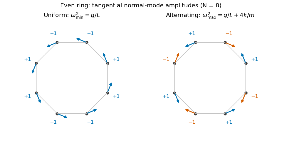
Original amplitude sketches for the lowest and highest modes of an even pendulum ring; arrows denote tangential displacements, not static positions
. Details. These are the even and odd pendulum-ring modes. For exact finite regular-polygon geometry with straight chord springs, the first-order spring extension includes a factor , so its squared contribution is multiplied by . That correction tends to one in the requested large- limit.
An odd ring. Perfect alternation cannot close after an odd number of steps. The two highest wave indices are instead and . They give a degenerate pair, represented by real sine and cosine standing patterns, withThe maximum is slightly below the even-ring limiting value, and the sign pattern must contain a gradual phase mismatch rather than exact alternation. The uniform lowest mode is unchanged, and there are still independent tangential mode directions.
Flow visualization and the idealization. A streamline is everywhere tangent to the instantaneous velocity field at one fixed time. A streakline is the locus, at one observation time, of particles that previously passed through a specified injection point. A marked particle's own trajectory is a pathline. These coincide geometrically in steady flow, but need not do so in an unsteady draining flow.
The intended ideal liquid is approximately incompressible and inviscid: viscosity and associated shear stresses are negligible on the scales and times being considered, the Mach number is small, and the density is effectively constant. This does not require zero vorticity; the initially rotating state is already a counterexample. It also does not justify ignoring viscosity in an arbitrarily thin boundary layer or at a real drain.
Spiralling flow and angular momentum. In an axisymmetric inviscid flow, pressure and gravity exert no torque about the vertical axis. A parcel therefore conserves axial specific angular momentum,The late, shallow remnant in the intended draining picture is supplied by parcels initially near the outer rim, so . The slow-drain angular-momentum amplification then givesThe assumption about the parcels' origin is necessary: torque conservation by itself does not assign to every parcel at every time.
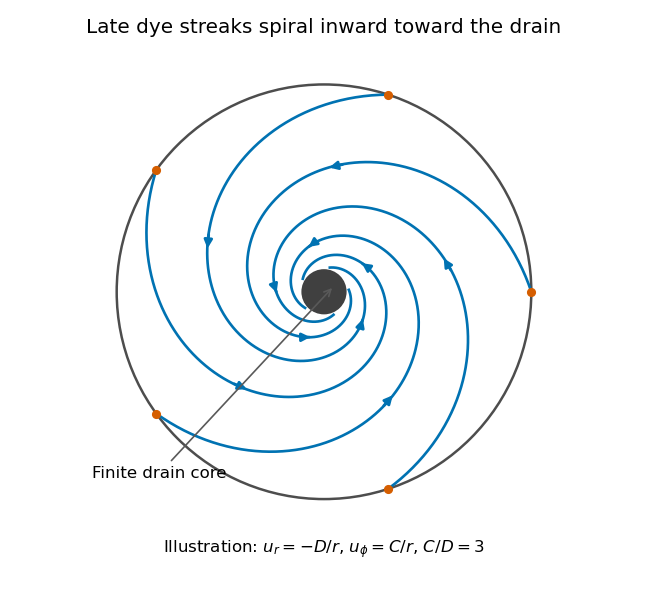
Original quasisteady illustration of inward-spiralling dye streaks outside a finite drain core; the azimuthal speed increases as the radius decreases
. Details. A continuous dye feed near the outer free surface produces inward spirals that wind increasingly rapidly near the drain. The figure uses a late quasisteady model, and with positive constants , giving . Its streaklines and streamlines approximately coincide over an observation interval short compared with the overall draining time. Strictly, individually marked particles at the initial surface trace pathlines, not a continuously injected streakline.
The free-surface depression. Let be the surface. Slow radial draining makes radial inertial corrections small compared with the azimuthal centripetal acceleration. The radial Euler equation and vertical hydrostatic equilibrium giveThus , with . Integrating from to the rim givesFor this becomesThe surface rises outward because the inward pressure gradient force must sustain the circular motion. The dimensions are metres, and the profile is not valid inside the finite drain or vortex core.
The terrestrial estimate. Use the vertical component of Earth's rotation as the ideal initial angular speed, . At Cambridge, taking and , this gives . Hence, for , and ,Taking the whole terrestrial angular speed rather than its local vertical projection would give about . The Cambridge estimate uses the projection appropriate to the vertical vortex. This very small head assumes terrestrial rotation supplies the only initial swirl; imposed residual rotation would change it quadratically.
Curl of the azimuthal velocity. For axisymmetric with no vertical dependence, the rotational part of the vorticity is vertical:The ideal quasisteady radial sink has no curl outside its core. The source's symbol denotes this vertical vorticity component, not the fluid's angular velocity. In general its magnitude is the absolute value of the bracket.
The two limiting states. For initial uniform rotation, , whereas the late approximation has . ThereforeThe late flow can have large angular velocity and nonzero circulation while being locally irrotational. The drain core is excluded from the domain of the velocity field.
What is actually conserved. Inviscid does not mean that each parcel's vorticity magnitude is fixed in three dimensions. For an incompressible barotropic liquid with conservative body forces, the vorticity equation isVertical compression of a material column changes its vorticity through vortex stretching, even while its volume is conserved by horizontal expansion. In the columnar shallow-layer limit, vorticity dilution in a shallow draining layer givesThus a remnant much shallower than its original column can have much smaller vertical vorticity. At finite depth there is generally a residual value; the exactly irrotational late profile is a leading limiting approximation, not an exact parcelwise conversion of nonzero vorticity to zero in finite time.
Kelvin's circulation theorem conserves circulation around a material loop, not around a fixed spatial circle. A loop whose original radius is near has circulation about , consistent with the late field. Fluid also leaves through the drain, so the remaining tank contents are not a fixed material system. If the calculation is expressed explicitly in the Earth-fixed rotating frame, the corresponding shallow-water potential vorticity is , with ; the conserved quantity involves absolute vorticity.
The units supplied for 130 indicate specific heat capacity, so the block's total heat capacity is . Treat it as constant, and the lake as a thermal reservoir at . The initial block temperature is .
Compute the block's entropy change using a reversible comparison path, even though the actual cooling is irreversible:The lake receives at constant temperature, soThereforeThis is entropy generated by cooling a finite body in a reservoir. The positive total is consistent with the Second law of thermodynamics, although the cooling block's own entropy decreases.
Initially and finally the block and lake are at the same temperature. After the falling block has come to rest, its lost gravitational potential energy has dissipated into internal energy of the lake and surroundings. In the idealization that all is ultimately thermalized in the lake at ,The block returns to its original thermal state, so its net entropy change is zero. Mechanical potential energy carries no thermal entropy that must be subtracted. ThusUse of gives the same three-significant-figure answer. Splashing and any temporary heating do not change this final-state balance if their mechanical energy is eventually dissipated in the same reservoir.
Three phase coexistence curves meet at the triple point, where ice, liquid water and water vapour have equal chemical potential. In the ordinary-pressure region, the low-temperature phase is ice, the high-pressure moderate-temperature phase is liquid, and the low-pressure high-temperature phase is vapour. The triple point is approximatelyBelow , warming stable ordinary ice crosses the sublimation boundary directly into vapour; there is no intervening stable liquid. Above , melting and then boiling can occur. The liquid–vapour curve terminates at the liquid-gas critical point, approximately and , beyond which there is no liquid–vapour phase boundary.
The distinctive feature is the negative slope of the ordinary ice–water melting line. The Clapeyron equation givesMelting increases entropy but reduces volume because ordinary ice is less dense than liquid water, so and . Increasing pressure consequently lowers the melting temperature locally. Sublimation and vaporization both increase volume and entropy, giving positive slopes. The following original schematic shows these signs; it is not a quantitative fit and omits the additional high-pressure ice polymorphs.
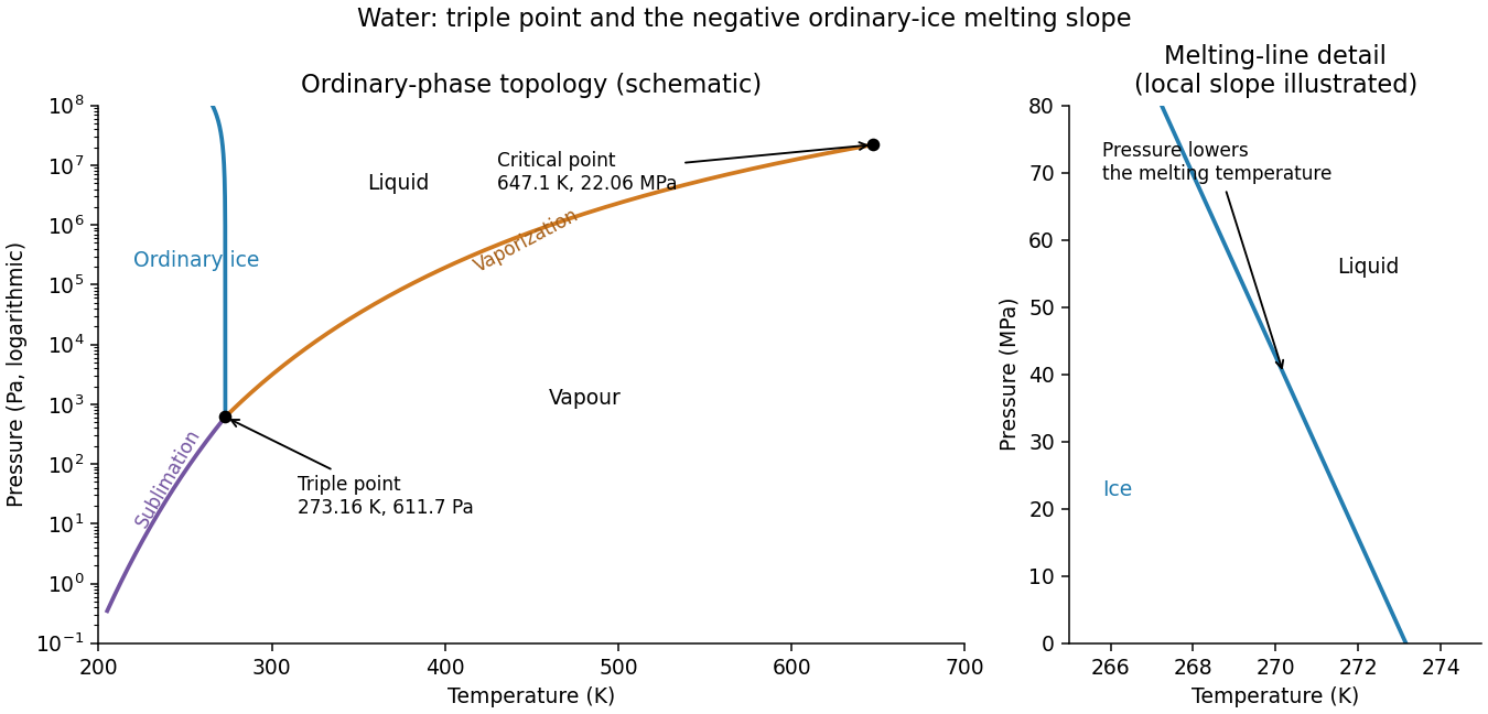
Schematic water pressure–temperature phase diagram with ordinary ice, liquid, vapour, triple point and critical point
. Details. Assume an air-filled or evacuated lossless electromagnetic waveguide, and a pulse bandwidth narrow enough to use its carrier's local group velocity. The longitudinal dispersion relation isIt givesHere , soThe phase velocity exceeds , but the pulse envelope travels at the subluminal group velocity; a moving constant-phase surface does not by itself transport information. Their product is . A broad pulse can distort because this waveguide is dispersive.
The original PDF calls a relative magnetic permeability while also specifying a nonmagnetic dielectric. These descriptions are inconsistent if read literally. The physically consistent interpretation of the notation is relative permittivity and relative magnetic permeability .
Let and let be the inner radius of the outer conductor. For line charge density , Gauss's law gives , henceThe magnetic field in the dielectric is . Its energy per unit length givesUsing ,These are the lossless coaxial line parameters, assuming negligible field penetration into the conductors. If the quoted radii instead referred to an outer diameter or if were intended, the data would need clarification; the stated dielectric and nonmagnetic assumptions support the interpretation above.
For an ideal electrical transformer, let . The reflected secondary load is . Matching a load to an source therefore requiresWith the generator replaced by its internal resistance, its resistance referred to the secondary isThis is the source output resistance relevant to matching and maximum power transfer.
To find the windings, use the inductance of a toroidal winding. The mean magnetic path is , the core area is and . ThusThe ideal secondary turn count is , giving the practical nominal designWith integer turns the irrational ratio cannot be exact: reflects the load as , an approximately resistance mismatch. These turn counts use the stated self-inductance; no operating frequency was specified from which to set a separate minimum inductance.
The condition must refer to the unloaded magnetizing reactance, not to the matched loaded input resistance. With ,The secondary self-inductance is , so its corresponding unloaded coil impedance satisfiesIf output impedance means this transformed coil reactance, is its minimum magnitude. It is distinct from the transformed source resistance. This is the magnetizing reactance and reflected resistance in a transformer distinction. A finite magnetizing inductance adds a parallel branch, , so exact purely resistive matching is an ideal large-reactance approximation; interpreting the loaded input itself as both and at least would be impossible.
In a homogeneous linear medium, write and . Without free charge or current, Maxwell's equations becomeTaking the curl of Faraday's law, using , givesTheir plane-wave solutions have and speed ; in vacuum this is . For a wave , the divergence equations give , while Faraday's law gives . Thus the fields and propagation direction form an orthogonal triad, with .
The two independent transverse electric components allow linear, circular and elliptical polarization of an electromagnetic wave. Their relative amplitudes and phase determine the polarization state. In a lossless nondispersive medium the energy density and energy flux areA travelling plane wave has equal electric and magnetic energy contributions and time-averaged intensity , where is its wave impedance and denotes peak electric-field amplitude. Reflection and refraction follow by imposing the electromagnetic boundary conditions. Frequency-dependent constitutive response introduces dispersion; conductivity introduces attenuation, so the simple real constant-speed result has a specified domain of validity.
A dielectric responds to an electric field mainly by displacing or orienting bound charges, rather than by sustaining a steady conduction current. The polarization density is electric dipole moment per unit volume. It creates bound chargeSeparating these charges from free charge motivatesFor an isotropic linear dielectric, , soThe electric susceptibility describes material polarization and is not the magnetic susceptibility. More generally it is a tensor and can depend on frequency, field strength and temperature.
Electronic polarization displaces an Electron cloud relative to its nucleus; ionic polarization displaces positive and negative ions; orientational polarization partially aligns permanent molecular dipoles against thermal disorder. For independent permanent moments of magnitude , weak-field orientational response gives when local-field corrections and interactions are negligible. This explains a common inverse-temperature contribution without asserting that every dielectric follows that law.
At a static interface, and the tangential electric field is continuous. Bound surface charge is already included through . For a homogeneous filled capacitor, , and a reversible linear dielectric stores energy density . At fixed voltage, insertion raises the stored field energy but the voltage source also supplies energy; force arguments must include that source. At fixed charge the capacitor energy instead decreases on insertion.
At frequencies too high for a polarization mechanism to follow the field, its contribution weakens. A complex permittivity represents dissipative dielectric loss as well as phase lag; the sign of its imaginary part depends on the time convention. Strong fields can cause nonlinear response or dielectric breakdown, beyond the reversible linear model.
In a homogeneous Ohmic conductor, . Combining this with Maxwell's equations givesFor a good conductor, , so conduction dominates displacement current. With time dependence and depth , take . ThenThe field is consequently proportional to : it both attenuates and changes phase with depth. The skin depth is the distance for amplitude to fall by ; power density falls as , so its attenuation length is .
Physically, changing fields induce currents whose magnetic field opposes penetration. Equivalently, after neglecting displacement current, magnetic diffusion obeys . Faster changes have less time to diffuse into the metal. Increasing frequency, conductivity or magnetic permeability reduces , provided the relevant material parameters remain applicable.
For a thick conductor the tangential surface electrical impedance is with the stated time convention and consistent field orientation. Its real part represents dissipative resistance per square. Current crowding near the surface raises the AC resistance of a wire when is small compared with its radius; thin strands and laminated magnetic cores reduce suitable eddy-current losses. When , the full complex propagation constant must replace the good-conductor approximation. In a magnetic metal the magnetic permeability can itself be nonlinear and frequency dependent.
A transmission line must be treated as a distributed circuit when its propagation time is significant on the signal timescale. Let denote resistance, inductance, leakage conductance and capacitance per unit length. Applying Kirchhoff's voltage law and Kirchhoff's current law to a short length gives the telegrapher's equationsFor a lossless line, . Differentiating again gives wave equations withThe travelling solutions can be written and . The minus sign for the backward wave is essential to power transport.
At a load , continuity of voltage and current gives the voltage reflection coefficientA matched termination absorbs the incident signal without reflection. An open circuit has and a short circuit has . Superposed incident and reflected waves produce standing waves. A sinusoidal lossless line of length transforms the termination intofor the convention. At a quarter wavelength, , allowing impedance transformation. A coaxial line supports a transverse electromagnetic mode whose ideal are calculated in A4. Its energy travels in the fields between conductors; the characteristic impedance is not the wire's DC resistance. Losses introduce attenuation and make the characteristic impedance and propagation constant complex.
Magnetization and field response. A magnetic material contains microscopic magnetic moments associated with Electron spin and orbital motion. The magnetization is magnetic dipole moment per unit volume. In SI the macroscopic fields satisfyHere separates free-current excitation from the material response. A uniform isotropic linear material has , givingThis constant scalar magnetic permeability model is useful only within its linear range. Crystals can have a susceptibility tensor; strongly magnetic materials depend on field and magnetic history. For a finite specimen the internal also includes its demagnetizing field. In a uniformly magnetized ellipsoid, along a principal axis, so sample shape affects the apparent susceptibility.
Diamagnetic and paramagnetic response. Diamagnetism is a weak negative susceptibility caused by induced orbital response opposing the applied field. It occurs in all matter but can be masked by larger positive contributions. Closed-shell materials such as bismuth or many organic compounds show it clearly. Ordinary diamagnetism is often only weakly temperature dependent; superconducting flux exclusion is a separate collective phenomenon and is not described by an arbitrarily small negative susceptibility.
Paramagnetism arises when available magnetic moments partially align with a field. Thermal disorder prevents complete alignment at weak fields. For independent localized moments of magnitude , the classical weak-field result iswhere the second expression uses in a weakly magnetic sample. Thus localized moments obey a Curie law in this regime. Quantum angular momentum changes the coefficient to the appropriate expression and gives saturation at strong field. Conduction Electrons instead exhibit Pauli paramagnetism: only states near the Fermi surface can change spin populations, so a degenerate gas has a nearly temperature-independent response. Its orbital diamagnetism must also be included for a full metallic susceptibility.
Collective magnetic order. Exchange interactions can favor parallel alignment, producing ferromagnetism below the Curie temperature. Iron, cobalt and nickel are familiar examples. A material may contain regions of spontaneous magnetization, or magnetic domains, while having little net external moment because the domains point in different directions. Applied fields move domain walls and rotate moments; at large fields the magnetization approaches saturation. Pinning and energy barriers make this process hysteretic. Remanence is the magnetization left after removing the driving field, and coercivity measures the reverse field needed to bring the chosen response back to zero.
The area of a closed – loop is the energy dissipated per unit volume per quasistatic cycle, , with positive dissipated magnitude. Consequently the magnetic permeability is neither one universal constant nor enough information to describe a ferromagnet: differential magnetic permeability , saturation and hysteresis all matter. Above the ordering temperature the spontaneous moment disappears, and a Curie–Weiss law is often an appropriate approximate paramagnetic description away from the critical region.
In antiferromagnetism, ordered opposing sublattices have equal moments and cancel macroscopically in the ideal compensated case. The order disappears above the Néel temperature. In ferrimagnetism, opposing sublattices have unequal moments and leave a net magnetization. Ferrites combine ferrimagnetic response with relatively high electrical resistivity, making them valuable when eddy-current losses would be substantial in a metallic core.
Electromagnets and engineering choice. A coil supplies free-current magnetomotive force . For a simple uniform magnetic path, Ampère's law gives and flux . A high-magnetic permeability soft magnetic core concentrates flux and reduces the current required for a given field. With an air gap ,Even a short gap can dominate the magnetic reluctance. The approximate attractive force across one uniform gap is , obtained from the field energy, with fringing neglected.
Soft magnetic materials have small coercivity and narrow hysteresis loops; they suit relays, electrical transformer cores and controllable electromagnets. Hard magnetic materials retain their magnetization and suit permanent magnets. Laminating metallic cores breaks large eddy-current loops; ferrites are useful at higher frequencies because of their resistivity. Increasing current cannot increase indefinitely through the linear formula: core saturation, coil heating and leakage limit performance. A good design selects material for the field amplitude, switching frequency and acceptable loss, rather than simply choosing the largest quoted magnetic permeability.
Let the rotating frame have origin acceleration and angular velocity relative to an inertial frame. For a vector referred to the moving axes, the transport rule isApply it twice to position. With rotating-frame velocity and acceleration ,Thus Newton's equation expressed in the rotating frame isThe added terms are translational, Coriolis, Euler and centrifugal fictitious forces. They reflect the frame's acceleration, rather than additional interactions with nearby objects.
The centrifugal force points outward from the rotation axis and, for constant , has potential . The Coriolis force is perpendicular to velocity, so does no work on the particle measured in that rotating frame; it changes direction rather than speed directly. The Euler force is present when the frame's rotation rate or direction changes.
On Earth, gravity and centrifugal acceleration combine into effective gravity. For slow horizontal motion at latitude , the vertical component of Earth's rotation gives Coriolis parameter : an initially northward motion deflects eastward in the northern hemisphere. This supplies a useful local explanation of rotating flows and Foucault precession. A bucket of rotating liquid illustrates the centrifugal potential: its steady free surface is an equipotential of , giving . These equations require a declared frame; adding a centrifugal force while retaining inertial-frame acceleration would count the same kinematic effect twice.
For a slender elastic beam undergoing small bending, cross-sections remain approximately plane and perpendicular to the centreline. At distance from the neutral axis, longitudinal strain is , where is curvature. Linear elasticity gives , so the bending moment has magnitudeHere is the second moment of cross-sectional area, not a mass moment of inertia. For width and depth in the bending direction, . The cubic depth dependence explains why a deep beam resists bending more effectively than the same material spread sideways.
For a uniform beam with transverse displacement , and bending energy is . Balancing transverse load yields the Euler-Bernoulli beam equation under a consistent sign convention. Supports specify values of deflection, slope, moment or shear; the equation alone does not fix the response.
Now apply a compressive end load . A small deflection shortens the axial projection by , so the total potential energy relative to the straight configuration isIts stationary equation isFor pinned ends, and the end moments vanish, so . The candidate shapes require . The first loss of stability is consequentlyAt smaller , the quadratic energy is positive; beyond this threshold the straight configuration no longer minimizes it. End restraint changes the threshold: clamped–clamped gives and clamped–free gives , equivalently an effective-length correction. A column buckles in the direction of smaller flexural rigidity. Euler buckling is a geometric instability within elastic response; yielding or crushing can occur first for a short thick strut. Large deflections, shear deformation and imperfections require refinements of the ideal slender-beam model.
Take a fixed sphere of radius in an unbounded incompressible inviscid fluid, with uniform velocity at infinity. Assume irrotational flow, so and incompressibility gives . Axisymmetry and the dipolar angular dependence of the far field suggestMatching the far field gives . The no-penetration condition then gives . ThusThe surface has stagnation points at its front and rear poles, while the equatorial speed is . Fluid slips tangentially past the sphere; imposing a no-slip condition would contradict this inviscid potential-flow model.
With gravity omitted or the hydrostatic pressure subtracted, steady Bernoulli givesAt the surface,The front–rear symmetry makes the integral of pressure force along the flow vanish: terms proportional to integrate to zero over the sphere. This is D'Alembert's paradox, not a prediction that real spheres have no drag. Viscosity creates boundary layers; separation and a wake break the fore–aft symmetry. Potential flow remains valuable for the outer velocity field when viscous regions are thin, but it cannot supply their drag by itself.
A spatially uniform external gravitational acceleration moves a body's centre of mass without stretching it. Tidal forces arise from the variation of that acceleration across the body. Let a distant mass lie at distance along unit vector , and let denote position relative to the body's centre. Subtract the centre's acceleration. To first order,The tidal tensor is . It stretches along the line to the source with eigenvalue and compresses in the two perpendicular directions with eigenvalues . Its trace vanishes outside the source, consistently with Laplace's equation for the gravitational potential.
After removal of the constant and uniform-acceleration terms, the tidal potential isAn ideal equilibrium ocean on a sphere of radius follows an equipotential of the body's gravity plus this perturbation. For surface gravity , the leading displacement isup to a constant fixing total water volume. The quadrupolar form produces bulges on both the near and far sides; the far-side bulge follows from differential acceleration, without postulating a repulsive gravitational force.
The Moon and Sun both raise terrestrial tides, with relative strength set mainly by , rather than by the total gravitational pull . Their contributions reinforce near new and full Moon to produce spring tides, and partly cancel near quadrature to produce neap tides. Earth's rotation relative to the tidal pattern gives a strong semidiurnal component in the simplest geometry. Real tide heights and timing depend on ocean depth, coastlines, basin resonances, Coriolis acceleration, friction and the declination of the forcing bodies. Tidal dissipation produces phase lags and torques, exchanging rotational and orbital angular momentum and gradually altering the spin and orbit. The equilibrium bulge is therefore a useful starting model, not an exact local tide forecast.
Inertia is a tensor. For a rigid body, distances between material points are fixed. Write each position relative to the centre of mass as , so its rotational velocity is . Integrating gives angular momentumThe rotational kinetic energy isThe inertia tensor is real and symmetric, so orthogonal principal axes diagonalize it. Angular momentum is parallel to angular velocity only along a principal axis, or within a subspace of equal principal moments. For translation plus rotation about the centre of mass, . Moving the reference to a parallel axis adds to the tensor, the tensor form of the parallel-axis theorem.
Euler's equations. The external torque about the centre of mass obeys . In body axes, the transport rule givesThe principal moments are constant in that frame, henceThese are Euler's equations. With zero torque, spatial angular momentum and kinetic energy are conserved, although the body components generally vary. For distinct moments, small perturbations about rotation around the largest or smallest principal moment oscillate, whereas those about the intermediate moment grow. This is the intermediate-axis instability.
A lamina. Choose the lamina's plane as . Then , so the normal is a principal axis, andThis perpendicular-axis theorem applies to a planar mass distribution; it is not a general identity for a three-dimensional body. Rotate the in-plane axes to diagonalize the remaining symmetric two-by-two block. For a uniform rectangular lamina with sides and mass , its central principal moments are , and . If , then : torque-free rotation about the long in-plane axis or the normal is stable, while that about the short in-plane axis is unstable. Coincident moments in a square require the degenerate, rather than strict intermediate-axis, case. Under a constraint to rotate only about the normal, the motion reduces to the scalar equation .
A symmetric top without torque. Let and . Euler's equations reduce toThus rotates at signed body-frame frequency , while the axial component stays fixed. The symmetry axis has constant angle to fixed spatial angular momentum. Indeed , soIt precesses in space about with angular speed . This spatial precession and the body-frame frequency describe different motions and should not be identified.
A heavy top. If a symmetric top is pivoted a distance from its centre of mass, gravity gives torque . Here the relevant moments are about the fixed pivot. The axial angular momentum and the vertical angular-momentum component are conserved, because gravity supplies neither an axial torque nor a torque about the vertical. Using tilt , precession angle and spin angle , its Lagrangian isEliminating the two conserved cyclic momenta leaves one-dimensional motion in an effective tilt potential; bounded oscillation in tilt is nutation. Steady precession at and fixed tilt satisfiesFor a rapidly spinning top on the slow branch, the first term is small andGravity then changes the direction of angular momentum rather than simply tipping the top straight down. The approximation fails near conditions where nutation or the fast-precession branch matters; the full equations retain those possibilities.
Pressure and its physical terms. Solving the molar Van der Waals equation for pressure givesThe excluded-volume parameter reduces the volume available for translational motion, raising the kinetic pressure relative to . The attraction parameter lowers the pressure because attractive interactions reduce the momentum transferred to the boundary. This mean-field model treats as temperature-independent material constants. For one mole, is the sample volume with the molar amount already fixed; has units of that volume and of pressure times volume squared.
volume dependence of entropy. The Helmholtz free energy has differential . Equality of mixed derivatives yields the Maxwell relationFor this derivative is , givingEquivalently, with a common reference volume understood inside the logarithm. The equation of state fixes this volume dependence, not the otherwise unspecified function of temperature.
Excess entropy at fixed volume and temperature. The ideal gas has . ThereforeIntegrate from infinite volume, where the entropy difference is specified to vanish:It is negative because excluding configurations reduces the accessible state count. It tends to zero as and has leading dilute limit . This is the entropy excess of a van der Waals gas.
Effect of attraction. Restoring a temperature-independent changes the pressure by , but not its derivative with respect to temperature. With the same infinite-volume entropy reference, it therefore does not change at fixed . This can also be seen fromThe attraction affects internal energy and the equilibrium volume, so it can affect entropy indirectly when different state points are compared. If were temperature dependent, its derivative would contribute directly to the entropy; that is outside the stipulated constant-parameter model.
Coexistence isotherm. Below the Van der Waals critical point, the formal homogeneous isotherm has a local minimum and maximum. Its middle branch has , hence negative isothermal compressibility, and is mechanically unstable. Portions of the negative-slope branches can be metastable rather than globally stable. The equilibrium isotherm replaces the loop between liquid volume and vapour volume by a constant saturation pressure . The two volume are fixed byThe Maxwell equal-area construction expresses equality of the two phases' chemical potentials. Intermediate total volume are mixtures: changing the vapour fraction changes total volume at the same pressure, rather than following the unstable homogeneous curve. The spinodals are the turning points of the formal isotherm; they are distinct from the coexistence endpoints.
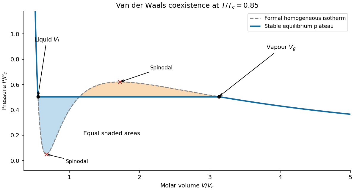
Original subcritical van der Waals isotherm showing the equal-area plateau, coexistence volumes and spinodals
. Details. Dense-phase volume at low temperature. At a general subcritical temperature, the two coexistence equations above must be solved together. For this equation of state the area condition is explicitlyThis supplies an exact implicit determination of the liquid volume even when a simple closed form is unavailable.
For the asymptotically low-temperature limit, put . The liquid is dense, , while the vapour is dilute, and . The area condition then givesThus the vapour volume grows exponentially in , and the saturation pressure is exponentially small. It is consequently consistent to neglect in the liquid equation to algebraic order in :Choose the root near , not the large-volume zero-pressure root:Expanding gives the leading requested dense-phase behavior,This is the low-temperature liquid volume of a van der Waals gas. Setting is an asymptotic approximation, not an exact coexistence condition at every temperature below . The figure illustrates generic subcritical coexistence; its finite-temperature liquid volume is determined by the full equal-area equations. The van der Waals liquid also ceases to be a realistic description at sufficiently low physical temperature, where other phases or quantum effects can matter.
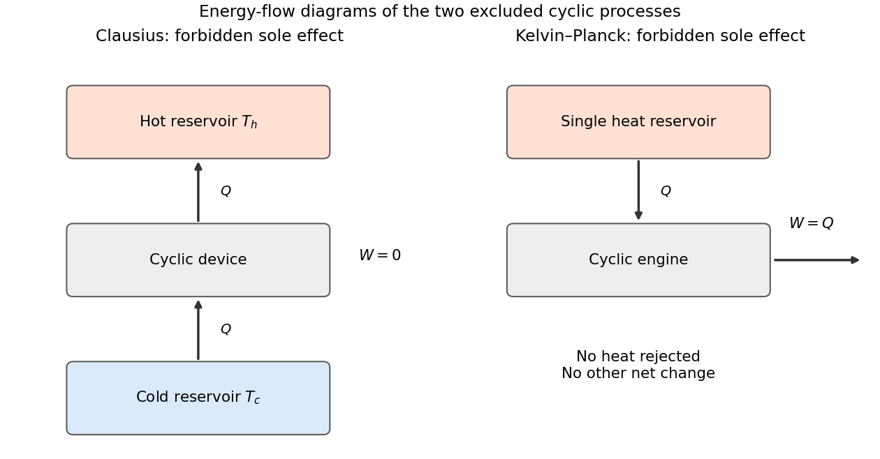
Two equivalent second-law statements. The Clausius statement of the second law forbids a cyclic device whose sole net effect is transferring heat from a colder reservoir to a hotter one. A refrigerator can make that transfer when supplied with work, so the sole-effect qualification matters. The Kelvin-Planck statement of the second law forbids a cyclic device whose sole net effect is drawing heat from a single reservoir and converting all of it into work. A heat engine can produce work when it also rejects heat to a colder reservoir.
The two statements are equivalent by combining a supposed violating device with an ordinary reversible engine or refrigerator: one can cancel one reservoir exchange and obtain a violation of the other statement. The following original schematic shows the forbidden sole effects, with arrows indicating energy flow.


Microscopic fluctuations. The second law is a macroscopic statistical law. A finite fluctuation can transfer a small heat amount from cold to hot, with reservoir entropy change . Such an individual event does not imply that a cyclic engine can extract systematic useful work from equilibrium. Entropy-decreasing trajectories become exceedingly improbable when the entropy involved is large compared with . Under suitable microscopic reversibility conditions, fluctuation relations quantify the relative probabilities of positive and negative entropy production and give nonnegative mean total entropy production. Thus a deterministic no-fluctuation reading has a limit at small scales or short times; the statistical second law remains applicable.
Maximum heating rate. Interpret the quoted as the maximum work-input rate to an ideal reversible heat pump. This interpretation is needed to obtain a heating rate larger than its electrical input; the wording does not explicitly distinguish input power from delivered heat. A reversible cycle satisfiesTherefore the heating coefficient of performance isWith and ,The additional heat comes from the outdoor reservoir; it is not produced by converting work into more energy than was supplied.
Lowest outdoor temperature. Let . The largest available heating rate is , while the house loses . Equilibrium can be maintained whenAt the limiting outdoor temperature,HenceThis is the indoor-temperature limit of a Carnot heat pump. It assumes the ideal pump retains its stated input-power capability over the operating range. Real heat exchangers require finite temperature differences and incur irreversibility, so the reversible result is an ideal upper performance bound.
Conventional heater. At this limiting outdoor temperature, the required delivered heating power is simply the house's heat loss:This is heat delivered to the house. The fuel-input power would be for heater efficiency . At the earlier outdoor temperature of , the required delivered heat would instead be ; the final question's reference temperature must be kept clear.
If is read literally as a maximum delivered heat rate rather than a work-input rating, the alternative answers are , , and a conventional heater delivering at that limit. Such a pump could not balance the stated house loss at . Both readings follow consistently once the ambiguous power rating is defined; the Carnot calculation above uses the work-input reading.
Configuration count. Choose the end-to-end direction as positive and let count rightward and leftward links. ThenA configuration is determined by choosing the positions of its leftward links, soThe counts must be nonnegative integers; in particular, allowed signed extensions occur in steps of . If distance means with neither direction selected, there are two corresponding sets for , adding a factor of two. That constant does not affect the tension. There is no excluded-volume penalty in this one-dimensional idealized count.
Entropy from the multiplicity. Put , so . Applying the leading Stirling's approximation to all three large factorials givesTerms subleading in , including logarithmic factorial prefactors, have been omitted consistently. Expanding near zero extension givesStretching reduces the number of available configurations and hence the entropy.
Tension and the range of Hooke's law. The model assigns no extension-dependent internal energy. At fixed temperature, the externally applied tension is . Differentiating the full leading entropy givesIt is the external force needed to oppose the chain's restoring entropic force. Only when can one put , yieldingThe paper's displayed linear law therefore requires this small-extension approximation, which is not explicitly stated in its premise . It is not the exact force law up to full extension. The entropic spring constant grows with temperature because stronger thermal disorder makes a given reduction in configurational entropy cost more free energy. This is the one-dimensional entropic chain force-extension relation.
A sparse number of backward links. Write , so and . Exactly,For fixed and large , each numerator factor approaches , givingMore precisely, the logarithm of the product is . A small relative error in the multiplicity requires ; merely need not make the omitted product close to one. The weaker sparse-link condition does suffice for the leading entropy density and leading high-extension tension. These are sparse backward links near full chain extension.
Tension in that limit. In the overlap regime , use Stirling also for :ThusThe full leading entropy would give , which has the same dominant logarithm when .
Approaching full extension. The continuum force law diverges logarithmically as , or . One must not literally apply Stirling to a zero factorial: at the discrete endpoint there is exactly one directed configuration, , and its entropy is zero. A continuous fixed-extension derivative is not defined at that endpoint.
An independent force-ensemble calculation makes the limiting physical statement precise. For applied tension , a link has partition function , giving the exact mean extensionIt approaches only as at positive temperature, and inversion reproduces the logarithmic force law for mean extension. In a real chain, bond extension or failure eventually replaces the ideal inextensible-link model.
Temperature as an equilibrium relation. Classical thermodynamics begins with the zeroth law of thermodynamics: thermal equilibrium is transitive. A thermometer can therefore assign a common empirical temperature to systems in mutual thermal equilibrium. Different thermometer properties initially give different monotone empirical scales; a resistance reading by itself does not define the absolute scale.
The Second law of thermodynamics provides a substance-independent thermodynamic scale. A reversible engine operating between reservoirs has a heat ratio depending only on their temperatures. One chooses absolute temperature so that , with the positive heat magnitudes. Its reversible efficiency is . Equivalently, reversible heat defines entropy through . For an equilibrium simple compressible system,Classical thermodynamics uses this relation without needing a microscopic account of entropy. A dilute-gas thermometer realizes an empirical scale approaching the thermodynamic scale after corrections for nonideal behavior.
Statistical meaning of the same derivative. In the microcanonical description, an equilibrium energy shell containing accessible states has . Its statistical temperature is consequentlyTo see why this is an equilibrium temperature, let two weakly coupled systems exchange a small energy while their total energy stays fixed. The combined multiplicity is . Maximizing its logarithm giveswhich is equality of the two inverse temperatures. Stability requires the total entropy maximum, not only stationarity. The overwhelmingly dominant macrostate in a large system therefore realizes the thermodynamic equilibrium condition.
A large reservoir gives a small subsystem the canonical probabilities , with . In that ensemble, and agree with macroscopic thermodynamic relations in their usual equilibrium regime. The equipartition identity for a classical dilute monatomic gas, , is a useful operational connection between microscopic motion and temperature, but is not a universal definition: quantum modes need not obey equipartition, and a system away from equilibrium need not have one temperature at all.
For finite systems one must specify the entropy convention and energy resolution; surface and fluctuation corrections can distinguish definitions that agree in the ordinary thermodynamic limit. Bounded-energy population-inverted systems can also have a negative entropy derivative and hence a negative statistical temperature. That possibility lies outside an ordinary positive-temperature ideal-gas thermometer; it does not mean temperature is merely an arbitrary average kinetic energy.
Obtaining the energy–temperature conversion. The Boltzmann constant connects entropy measured in with the dimensionless logarithm of a state count. Historically it could be determined from the ideal gas law : measure the molar gas constant and independently determine the Avogadro constant , then obtain . The independent particle-number determination matters; using alone would not fix energy per particle.
An electrical method uses Johnson-Nyquist noise. A resistor of resistance at known temperature has, in the classical range , a one-sided open-circuit voltage-noise spectrum . Over a calibrated flat bandwidth ,A practical measurement uses an equilibrium resistor, a calibrated low-noise amplifier and a known transfer function, subtracts or independently characterizes amplifier noise, and replaces a nominal bandwidth by the actual effective noise bandwidth. Varying temperature and fitting the mean-square voltage is more informative than treating one amplified voltage sample as the thermal variance. Other primary methods relate temperature to sound speed in a dilute gas or to calibrated particle diffusion and mobility.
There is a historically relevant unit-definition qualification: by the date of this exam, the revised SI had already taken effect on 20 May 2019. The kelvin is now defined by fixingThe same experiments now realize or compare thermodynamic temperatures using this fixed constant, whereas historically they measured the conversion constant on an independently defined temperature scale. The physical distinction between equilibrium temperature and microscopic state counting is unchanged.[ref]
https://www.bipm.org/en/measurement-units/. BIPM, SI definitions effective from 20 May 2019 and fixed Boltzmann constant
Articles by others on the same topic
There are currently no matching articles.