Use a real, even interaction . Let and . In the Bogoliubov theory expansion, keep terms with zero or two noncondensed operators. The zero-momentum term gives . The terms with two noncondensed operators giveHere is the direct condensate interaction and is its exchange contribution. At fixed total particle number, , soThe second term cancels the direct normal term. Adding the kinetic energy yields the number-conserving Bogoliubov quadratic HamiltonianThe constant is the condensate mean-field theory interaction energy; the normal term describes moving a particle out of the condensate, while the anomalous term creates or annihilates an opposite-momentum pair by exchanging two particles with the condensate. Total particle number remains fixed in the underlying theory; the condensate amplitudes in this notation are treated as classical amplitudes.
For condensate fluctuation power counting, put . Formal interaction-amplitude counting gives , cubic terms and quartic terms ; these are not uniform bounds on individual modes. Thus the latter are down by and relative to the quadratic interaction terms. The correction is relative . Homogeneity eliminates terms linear in nonzero-momentum operators. Small depletion and weak interactions, not low temperature alone, justify the truncation. [ref]
Lecture Notes for Quantum Matter by Steven H. Simon. §4.5, Bogoliubov expansion; fixed-number cancellation derived above
For each opposite-momentum pair use the Bogoliubov transformationEquivalently , , with . The identity preserves the canonical commutation relation. Vanishing anomalous terms require , and hence the Bogoliubov quasiparticle dispersion isSubstitution and normal ordering giveThis is the requested form after putting each inside the oscillator term. By momentum-pair counting in bosonic diagonalization, all sums cover the full nonzero-momentum set; no further factor of two is needed. The bosonic Bogoliubov zero-point shift combines the two vacuum sums before taking a continuum limit.
If smoothly, the low-energy excitations are gapless phonons:For contact repulsion, the healing length separates this regime from the particle-like regime . Stability requires for every nonzero mode. A general momentum-dependent interaction need not share the contact model's entire curve. An unregularized contact model also makes the vacuum-energy shift ultraviolet divergent; a physical finite-range interaction or scattering-length renormalization is needed for that absolute ground-state energy.
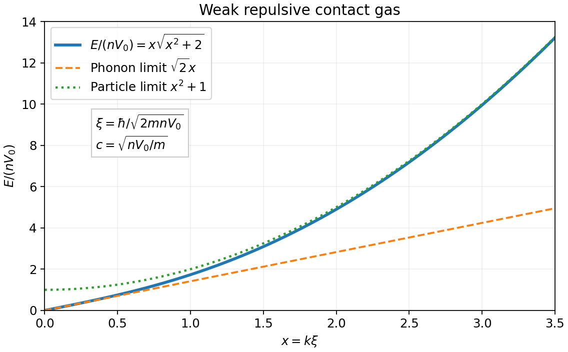
In the Bogoliubov quasiparticle vacuum, , but the inverse Bogoliubov transformation gives . Consequently the quantum depletion of a Bose condensate isThis expression assumes zero temperature. At nonzero temperature, thermal Bogoliubov quasiparticles add to the depletion:Thus the printed formula is the quantum contribution, or a low-temperature approximation when the thermal contribution is negligible. It is nonnegative for a stable quadratic Hamiltonian and vanishes in the noninteracting zero-temperature limit.
A periodic harmonic chain with masses , spacing and nearest-neighbour spring constant hasHamilton's equations give . The discrete Fourier transform , , with in one Brillouin zone, diagonalizes the quadratic form:The harmonic-chain normal-mode reality condition means , not that and are independent real coordinates. For canonical quantization, impose , equivalently . For setThen the quantum harmonic chain is a set of independent phonon oscillators:The centre-of-mass zero mode of a harmonic chain is the free coordinate , with ; it cannot be normalized by dividing by . Retaining it giveswith the corresponding momentum expansion and uniform term . The nonzero modes alone give the site commutator ; the uniform term supplies the missing . Each oscillator occupation is a nonnegative integer, and adding one phonon costs and crystal momentum modulo a reciprocal-lattice vector. [ref]
Applications of Quantum Mechanics by David Tong. §4.1.1, printed pp.103–105, monatomic-chain normal modes and quantization
In the continuum limit of a harmonic chain, , andThe wave equation and linear low- dispersion relation follow. The lattice gives an ultraviolet cutoff; the acoustic approximation does not reproduce the zone-edge flattening.
With the centre of mass fixed, the oscillator partition function and Bose-Einstein distribution areFor a long chain, above its finite-size level spacing and below the zone-edge scale, integrating the two acoustic propagation directions gives . At high temperature each retained oscillator instead contributes to the heat capacity.
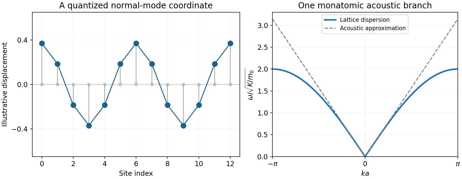
Original monatomic-chain mode sketch and its acoustic lattice dispersion
. Source. Details. For , divide elapsed time into slices and apply the Trotter product formula. Inserting complete position and momentum bases gives the regulated phase-space path integralThe endpoint values are , . Each Gaussian momentum integration in a phase-space path integral can be performed explicitly, leaving the configuration-space path integralIts measure is the time-sliced limit of , with the usual infinitesimal convergence prescription. The integral sums amplitudes, not positive classical probabilities. Operator ordering remains part of the time-slice definition. Expanding a short-time kernel recovers the Schrödinger equation; composing kernels reproduces the time-evolution operator.
In the classical limit, rapid phase cancellation suppresses paths away from stationary action. Varying with fixed endpoints gives . The semiclassical result sums the classical-path phases multiplied by fluctuation functional determinants; for a quadratic Hamiltonian the fluctuation integral is Gaussian and this expansion is exact.
For quantum statistical mechanics, continue by a Wick rotation. The Euclidean action and thermal trace giveThe trace closes position-space paths. In a many-particle trace one also sums over endpoint permutations with the appropriate exchange signs. In a coherent state field formulation, bosonic fields are periodic and fermionic coherent states instead give antiperiodic Grassmann fields, hence bosonic and fermionic Matsubara frequencies and . [ref]
Physics 215C: Quantum Field Theory, Part 3 by John McGreevy. §§3.1–3.2, coherent-state time slicing and trace boundary conditions
The quantum-to-classical imaginary-time mapping views a local -dimensional quantum problem as a classical-looking field theory in dimensions, with imaginary-time extent . A genuine classical probability interpretation additionally requires a nonnegative weight; fermion signs and Berry terms can obstruct it.
For a smooth potential in the high-temperature or small- limit, imaginary-time paths fluctuate only over the thermal de Broglie wavelength . If this is short compared with the potential's variation scale, the diagonal free kernel givesThis classical phase-space limit of the thermal kernel is the classical phase space partition function for one degree of freedom. A dilute identical-particle gas also needs its factor; when exchange is appreciable, classical statistics fails. As a check, a single quantum harmonic oscillator gives , precisely the classical phase-space integral.
For conventional superconductivity, an attractive interaction pairs opposite-spin fermions. A complex pairing Hubbard–Stratonovich transformation introduces a Cooper pair field . The fermionic fields then appear quadratically, giving the pair-field effective action of a superconductorThe trace convention counts each independent spin-pair block once. The uniform saddle is the BCS gap equation; the fermionic excitations have in the fully gapped case. A slow-field expansion near the transition yields Ginzburg-Landau theory of superconductivity. Normalize its pair field so is an effective pair density, with pair mass and signed charge :For , the uniform minimum has , with arbitrary constant phase. Writing separates the amplitude mode from the phase. The local potential has curvature term and coherence scale . A neutral condensate has a gapless phase Goldstone mode when suitable dynamics is included.
The charged theory is invariant underThe gauge-invariant condensate momentum is . Only and enter physical phase dynamics. At nearly constant amplitude, varying givesFor a smooth phase, taking the curl and using Ampère's law gives : the Meissner effect screens a static bulk magnetic field over the London penetration depth . In a gauge with , the phase stiffness is a quadratic term in , the superconducting version of the Higgs mechanism.
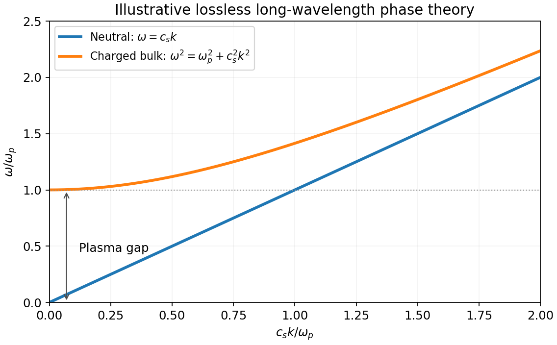
To identify the dynamical mode, a simple lossless long-wave superconducting phase-density action isHere is the pair compressibility coefficient. Eliminating the longitudinal electric potential givesThus the neutral sound mode becomes a gapped longitudinal plasma oscillation; transverse electromagnetic waves acquire in this simple bulk model. This redistribution of the phase degree of freedom into electromagnetic collective modes is the Anderson-Higgs mechanism in a superconductor. Local gauge symmetry is a redundancy, not an independently observable symmetry whose breaking creates another massless particle. [ref]
Physics 215C: Quantum Field Theory, Part 3 by John McGreevy. §2.3, superconductors, superfluids and gauged phase dynamics
The static functional alone does not determine a frequency or damping rate. The displayed mode dispersions require the added dynamical assumptions; real screening, normal carriers, boundaries and dissipation modify them. The amplitude fluctuation is distinct from the phase mode and is not removed by the gauge choice.


Use and dimensionless spin operators. At one site, the canonical anticommutation relations imply the on-site spin-square normal-ordering identityIndeed the empty and doubly occupied states have spin zero, while either singly occupied state has . Thus the interaction in normal-ordered form is . There is no residual chemical-potential shift: that contraction has cancelled.
Insert fermionic coherent state resolutions between imaginary-time evolution factors. With and , the grand-canonical coherent-state action isThe independent barred and unbarred Grassmann variables satisfy antiperiodic boundary conditions at . Adjacent time-slice labels in the normal-ordered symbol fix the continuum prescription and thermal normalization. The interaction coefficient is , not the of a differently normalized Hubbard model.
Expand the Grassmann fields in fermionic Matsubara frequencies . For , the Grassmann Gaussian integral factorizes into thermal fermionic one-level thermal determinants:Each factor counts the empty and occupied states of one spin orbital. Equivalently, the regularized Matsubara sum gives the logarithm of that factor; the raw infinite determinant requires thermal normalization of a fermion determinant. ThereforeThe printed is the grand potential , because the trace contains . The Helmholtz free energy at fixed mean particle number is .
Define the Grassmann spin density . The Pauli matrices and Grassmann reordering giveFor example ; each of the other two components gives the same result. For , complete the square independently at each site and time slice:This normalized spin-vector Hubbard–Stratonovich decoupling yieldsThe auxiliary bosonic quantum field is real and periodic, while the fermionic fields remain antiperiodic. All three vector components are required to reproduce the original interaction; replacing this exact transformation by a single-component identity would change its coefficient.
For the uniform mean-field approximation field , the inverse fermion propagator is diagonal in momentum, frequency and spin: . The Grassmann Gaussian integral therefore givesHere denotes the residual uniform-field measure; integration over its orientation only affects a nonextensive prefactor. HenceThe exchange field separates the two spin bands by . Integrating out the fermions is exact for a specified auxiliary field; restricting that field to be constant is the mean-field approximation.
Differentiate the uniform effective action:To reproduce the printed coefficient, define the spin-summed density of states per site byThe saddle-point approximation then givesThe uniform spin field and magnetization obey for occupations per site. If a one-spin density of states were used instead, the factor would be absent. The spin field is an energy, rather than directly a magnetic moment.
The constant term in the spin sum cancels. Linearizing the saddle point equation givesThe paramagnetic auxiliary-field curvature isConsequently the Stoner criterion for the loss of local paramagnetic stability isThe printed uses energy measured from the Fermi level. For a smooth density of states, becomes a narrow unit-area peak at ; a singular density of states or appreciable temperature requires the integral form. The curvature establishes local instability, not the order or location of every possible thermodynamic transition.
With exact spin-rotation symmetry, itinerant ferromagnetism selects a magnetization direction. The two broken transverse generators form one quadratic type-B Goldstone boson, a long-wave ferromagnetic magnon with . Longitudinal amplitude motion is not symmetry-protected to be gapless. In a metallic ordered state, particle-hole excitations remain near each surviving exchange-split Fermi surface; these are distinct from the collective magnon. The itinerant spin-flip particle-hole continuum starts at exchange scale at in this simple mean-field spectrum, while its finite- boundaries differ. Spin anisotropy, spin-orbit coupling or an external field can gap the transverse mode; none is present in the stated model.
Articles by others on the same topic
There are currently no matching articles.