Protein primary structure is the ordered amino acid sequence of a polypeptide, linked by covalent peptide bonds. The approximately planar peptide bond restricts local geometry, while backbone torsion angles give conformational freedom subject to steric exclusion. Protein secondary structure comprises local backbone arrangements, especially the alpha helix, with backbone hydrogen bonds between residues i and i+4, and the beta sheet, whose strands are joined by backbone hydrogen bonds. Turns and loops connect these elements. Protein tertiary structure is the full three-dimensional organization of a single chain, often including several protein domains. Protein quaternary structure is the arrangement of multiple chains in a protein complex.
Protein folding is governed by the Gibbs free energy of the chain together with its solvent, not by the chain's energy alone. Folding reduces the chain's conformational entropy, but can gain solvent entropy through the hydrophobic effect, burying nonpolar side chains away from water. Favorable hydrogen bonds, Van der Waals forces, electrostatic interactions and sometimes covalent disulfide bonds stabilize particular structures. Steric repulsion prevents atomic overlap. At fixed temperature and pressure, the native ensemble is favored when its total ΔG=ΔH−TΔS is lower than competing ensembles. The balance depends on the solvent, pH, salt and ligands. Molecular chaperones help avoid aggregation or kinetic traps; a stable fold is not a perfectly rigid conformation, and some proteins have disordered regions.
For a soluble globular protein, a typical pattern is a nonpolar core and a polar, hydrated surface. A transmembrane protein instead presents nonpolar side chains to the hydrocarbon interior of the lipid bilayer. Membrane-spanning alpha helices satisfy their polar backbone groups through internal hydrogen bonds; a roughly membrane-thickness helix commonly contains about twenty residues, depending on tilt and bilayer thickness. Multiple helices can enclose polar channels or binding sites. Membrane-spanning beta barrels likewise expose mainly nonpolar groups outward towards lipid while arranging backbone hydrogen bonds between strands and often lining an aqueous pore with polar groups. Exposed loops and domains contacting water can resemble soluble proteins. Not every membrane-associated protein spans the membrane: peripheral attachment and lipid anchoring are distinct possibilities.
The organizing distinction is the environment of each surface: water favors accessible polar groups, while the membrane core favors outward-facing nonpolar groups. Buried polar groups can still be essential to a transport pathway or catalytic site.
ATP synthase couples downhill proton motion across a cell membrane to synthesis of ATP from ADP and inorganic phosphate. Its membrane-embedded Fo sector contains an a subunit with offset proton-access half-channels and a rotating c-subunit ring. Reversible protonation of sites on the ring permits rotation relative to the stationary a subunit. The central rotor transmits this motion through the γ shaft to the soluble F1 head. A peripheral stator holds the head relative to the membrane sector. The common bacterial schematic has an α3β3 head, catalytic sites mainly on the three β subunits, and a central γ/ϵ rotor; accessory stator components depend on the organism.
The binding-change mechanism cycles the catalytic sites between open, loose-binding and tight-binding conformations. Rotor orientation changes their affinities for ADP, phosphate and ATP; the sites operate out of phase. Tight binding favors formation of bound ATP, and mechanical rotation changes the conformation to permit product release. In the ideal tightly coupled cycle, one revolution gives three catalytic turnovers:The proton count is not universally fixed: an ideal ring with nc proton-carrying subunits gives nc protons per revolution and nc/3 protons per synthesized ATP, before additional transport costs.
3 ATP per 360∘,1 ATP per 120∘.
For a proton moving from side 1 to side 2, its molar electrochemical potential change isThe chemical gradient and membrane electric potential difference together supply the proton-motive force. Synthesis requires the proton free-energy release to meet the positive Gibbs free energy of ATP synthesis. The coupling is reversible: isolated F1 supplied with ATP can hydrolyse it and rotate its shaft, while the intact enzyme can use hydrolysis-driven rotation to pump protons against their gradient. The sketch is structural and schematic; it does not reconstruct the absent stepping trace.
ΔμH+=RTlogaH+,1aH+,2+F(ψ2−ψ1).
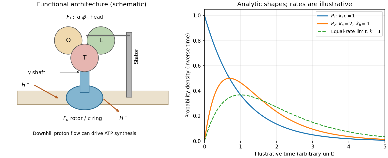
ATP synthase architecture and the two derived dwell-time distributions
. The structural panel shows a membrane rotor, shaft, stator and three catalytic sites. The distribution panel uses explicitly illustrative dimensionless rates, not values read from the absent source stepping plot. Details.Let S1(t) be the probability that an ATP-waiting state has not yet bound a substrate molecule. A constant bimolecular binding coefficient k1 at fixed ATP concentration c gives a pseudo-first-order hazard λ=k1c. Thus S˙1=−λS1, S1(0)=1, and the waiting-time distribution isThe probability density function starts at k1c and decreases exponentially. Increasing c shortens the waiting time in inverse proportion. This supports one rate-limiting ATP-binding event before the associated motion, rather than a concentration-independent chemical delay.
P1(t)=−S˙1(t)=k1ce−k1ct,t≥0,⟨t1⟩=k1c1.
For the second delay, consider sequential independent first-order transitions A⟶kaB⟶kbC. Their dwell times have exponential distributions. The total waiting time is their sum, so convolution givesIt is normalized, symmetric under exchange of ka,kb, and hasUnlike one exponential delay, it vanishes at t=0, rises initially as kakbt, reaches a maximum at tmode=log(ka/kb)/(ka−kb) and eventually decays at the slower rate. For equal rates the continuous limit is P2(t)=k2te−kt, an Erlang distribution with mode 1/k. If one rate is much faster than the other, the observed long-time behavior approaches one exponential. The sketch in the preceding section displays these shapes using arbitrary specified rates.
P2(t)=∫0tkae−kaskbe−kb(t−s)ds=ka−kbkakb(e−kbt−e−kat),t≥0.
⟨t2⟩=ka1+kb1,Var(t2)=ka21+kb21.
The simplest catalytic cycle compatible with the fits therefore contains an ATP-dependent binding delay and at least two resolvable ATP-concentration-independent kinetic events. Hydrolysis, product release and conformational changes are possible microscopic assignments, but the two-rate fit alone does not uniquely identify them or the order of ka and kb. If each complete 120∘ cycle contains these three waits and step durations are negligible, its mean duration is (k1c)−1+ka−1+kb−1 and the mean revolution rate is the inverse of three times this duration. Multiple catalytic sites can cooperate during that cycle.
TODO: the source PDF's stepping plot is absent. Its individual substep angles, numerical timings and the mapping of plotted dwell labels onto the larger or smaller angular movement cannot be read. The surviving text establishes only the 120∘ total step and the existence of a larger and a smaller substep. No numerical rate, missing angle or plotted label is inferred from a different experiment. The distribution derivations and the concentration-dependence inference above are independent of that illustration.
Write the one-dimensional random walk endpoint as xm=∑j=1mξj, starting at the origin. Assume unbiased, independent increments, each with ⟨ξj⟩=0 and ⟨ξj2⟩=Δ. Expanding the square givesIndependence makes each cross expectation ⟨ξi⟩⟨ξj⟩=0. ConsequentlyUncorrelated increments with the same second moments would suffice. Unbiasedness alone does not remove correlations: persistent or anticorrelated steps need not satisfy this result. The symbol Δ is already the mean-square step size, with units of length squared.
⟨xm2⟩=∑j⟨ξj2⟩+2∑i<j⟨ξiξj⟩.
⟨xm⟩=0,⟨xm2⟩=mΔ.
Let C(x) be the particle number density, U(x) the conservative potential energy and F=−dU/dx the applied force. In the overdamped regime a viscous drag coefficient ζ gives drift velocity vd=F/ζ. Combining this drift with Fick's first law gives the number fluxAt thermal equilibrium, the Boltzmann distribution is Ceq∝e−U/(kBT), so dCeq/dx=FCeq/(kBT). Setting its net flux to zero yieldsThis is the Einstein diffusion relation. The derivation assumes a dilute equilibrium suspension, uniform temperature, linear drift response and a well-defined long-time diffusion coefficient. With a nonzero conservative force, the full transport equation includes drift; the force-free equation in the next section describes spreading without that drift.
J=−DdxdC+ζFC.
0=FCeq(ζ1−kBTD),D=ζkBT=μkBT,μ=ζ−1.
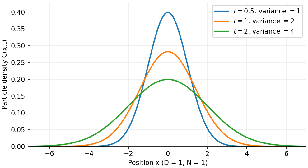
For constant D and no drift, particle conservation and Fick's first law give the one-dimensional diffusion equation ∂tC=D∂x2C. For C=At−1/2e−x2/(4Dt),so direct substitution verifies the equation for t>0. The Gaussian integral fixes the normalization:This is the heat kernel for a point release, with C(x,0)=Nδ(x) in the distributional limit. It remains centered at zero while its width grows as t1/2 and its peak falls as t−1/2. To compute the second moment, set y=x/4Dt:using ∫y2e−y2dy=π/2 over the whole real line, obtained by integration by parts.
∂tC=C(−2t1+4Dt2x2),∂x2C=C(−2Dt1+4D2t2x2),
∫−∞∞Cdx=A4πD=N,C(x,t)=4πDtNexp(−4Dtx2).
⟨x2⟩=N1∫x2Cdx=π4Dt∫−∞∞y2e−y2dy=2Dt,
If the mean number of independent unbiased jumps in time t is ⟨m⟩=ft, conditioning on m gives ⟨x2(t)⟩=Δ⟨m⟩=fΔt. Matching it to the continuum diffusion result yieldsFor fixed-magnitude steps a, Δ=a2. The equality of second moments also holds for Poisson jump times independent of the increments; a Gaussian continuum approximation additionally requires many steps and finite step variance.
D=2fΔ.


Ancestors (9)
- 2012
- Past exam of the short options paper shared by Prelims and Parts A and B of the physics course of the University of Oxford
- Short options paper shared by Prelims and Parts A and B of the physics course of the University of Oxford
- Physics course of the University of Oxford
- Undergraduate course of the University of Oxford
- Course of the University of Oxford
- University of Oxford
- List of universities
- Home
Discussion (0)
New discussionThere are no discussions about this article yet.
Articles by others on the same topic (0)
There are currently no matching articles.