The Stokes–Einstein relation connects thermal diffusion with dissipative mobility. For a dilute suspension of isolated rigid spheres of hydrodynamic radius in an unbounded Newtonian fluid of viscosity ,where is translational drag coefficient, diffusion coefficient and absolute temperature. Stokes drag supplies under no-slip, continuum, low-Reynolds-number conditions. The Einstein diffusion relation is more general than that particular spherical drag law.
A short equilibrium argument explains the connection. Let a weak external potential exert force , so drift velocity is . The number flux is . A Boltzmann distribution has ; requiring zero equilibrium flux fixes . thermal fluctuations and viscous dissipation are therefore linked, rather than independent adjustable effects. The original theory also relates diffusion to measured random displacements.[ref]
On the Movement of Small Particles Suspended in a Stationary Liquid Demanded by the Molecular-Kinetic Theory of Heat by Albert Einstein. Sections 3–5, printed pages 9–18 in the linked translation: equilibrium flux balance, spherical drag and displacement variance
On times long compared with momentum relaxation, an isotropic diffusing sphere hassingle-particle tracking can measure the slope. Alternatively, dilute single-scattering dynamic light scattering measures a field correlation ; the corresponding intensity-correlation excess is proportional to . The scattering wavenumber and the distinction between field and intensity decay must be retained.
A Stokes-Einstein experimental consistency test independently measures temperature and solvent viscosity, uses a narrow distribution of inert spheres, checks decay rate proportional to or displacement variance proportional to time, and extrapolates toward infinite dilution. Subtract drift, account for wall-enhanced drag, and verify that aggregation is absent. Tracking additionally needs spatial calibration and correction for finite exposure and localization precision. At finite concentration, collective diffusion is not automatically the single-particle self-diffusion in the equation. A hydrodynamic radius is not generally identical to a polymer radius of gyration; nonspherical particles, slip or viscoelastic solvents require a different mobility model.
polymers at interfaces balance favorable surface contacts against lost conformational entropy and interactions among neighboring chains. At an attractive solid–liquid interface, an adsorbed polymer train consists of consecutive bound segments. An adsorbed polymer loop leaves the surface and returns to it, while an adsorbed polymer tail extends to a free chain end. A chain can contain all three, so adsorption does not imply a completely flattened molecule. Surface affinity, solvent quality, persistence length, chain length and concentration control the balance and the resulting segment-density profile.
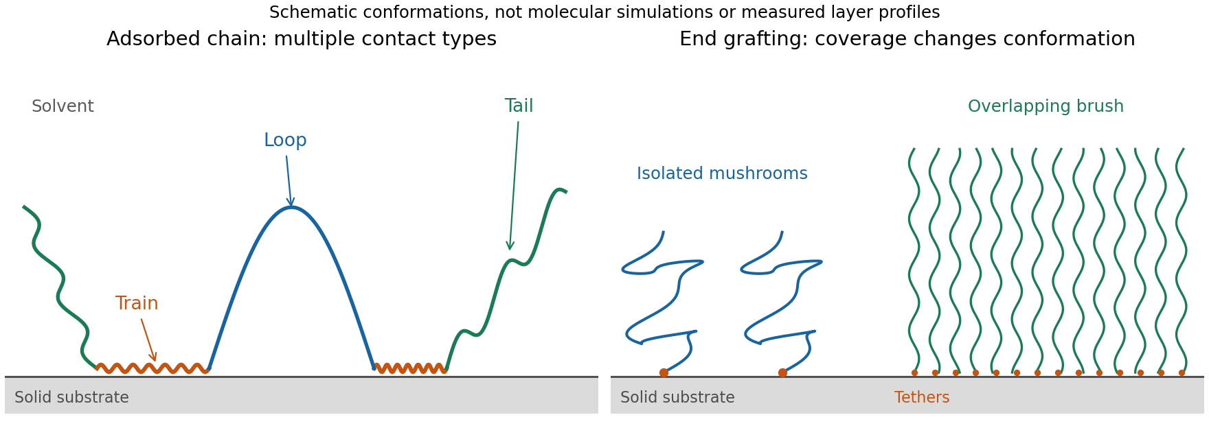
Original schematic of adsorbed trains, loops and tails, and the crossover from isolated grafted mushrooms to an overlapping polymer brush
. Details. 
adsorption gains energy of order per bound segment but reduces the number of accessible chain configurations. Weak adsorption can be described through adsorption blobs whose thickness exceeds the statistical segment length; each blob loses an energy of order through confinement. Stronger attraction generally creates more contacts and a more compact layer, while loops and tails can still dominate its outer extent. A measurement of adsorbed mass alone therefore does not determine layer thickness or conformation.
End-grafted chains are different: their attachment is fixed at one end. At grafting density , the mean lateral spacing is . At low coverage the chains behave as isolated polymer mushrooms. The polymer mushroom-to-brush crossover occurs when . At higher coverage in a good solvent, crowding makes chains extend away from the surface. A free-energy balance per chain,combines stretching entropy with repulsive excluded volume . Minimization gives , orThis is a scaling result with an undetermined order-one coefficient, valid for overlapping chains stretched below their contour length. In a compact poor-solvent layer, a roughly fixed internal polymer volume fraction instead gives .
Small-angle neutron scattering on end-grafted polydimethylsiloxane layers on porous silica has distinguished the good- and poor-solvent density exponents. The chemical system and scattering contrast matter: changing solvent quality should be separated from changing graft coverage, chain molar mass or adsorption strength.[ref]
Characterization of the brush regime for grafted polymer layers at the solid-liquid interface by P. Auroy and others. Physical Review Letters 66, 719–722 (1991), abstract: actual polymer/substrate system, neutron-scattering method and the two thickness scalings
An interface can also localize chains of a block copolymer when its blocks prefer different media. Such layers change interfacial tension and can stabilize dispersed droplets or particles through steric repulsion. Overlapping layers in a good solvent cost osmotic and conformational free energy; incomplete adsorption can instead produce polymer bridging between particles. Nonadsorbing chains can cause depletion attraction. Thus the presence of a polymer does not by itself guarantee stabilization.
A viscoelastic material stores part of the work of deformation and dissipates part. In the linear regime its stress depends on the strain history, not just the instantaneous strain or shear strain rate. For simple shear, a causal relaxation modulus gives . A sudden strain then probes stress relaxation, while a constant imposed stress probes material creep; these are different experiments.
For steady sinusoidal strain use the convention and complex amplitudes. The complex viscoelastic modulus isso . The storage modulus is the in-phase elastic component. The loss modulus multiplies the component in phase with shear strain rate; stress leads strain by . The loss tangent is when .
Multiplying stress by shear strain rate and averaging gives . Hence the dissipated energy per oscillatory shear cycle isThe elastic contribution returns its work over the cycle. A passive material has nonnegative dissipation, which fixes the sign of the loss term in the chosen Fourier convention. This complex viscoelastic modulus is a response function, not the mathematical absolute value of a complex number.
A Maxwell model places a spring of shear modulus in series with a dashpot of viscosity , so the strains add at common stress:The Maxwell fluid dynamic modulus isAt the response is predominantly viscous, and . At it approaches the elastic plateau . The two moduli cross, and reaches its maximum, at . A Kelvin-Voigt model instead has the spring and dashpot in parallel, giving and no fluid-like zero-frequency terminal flow. Real materials often need a spectrum of relaxation times rather than one Maxwell time.
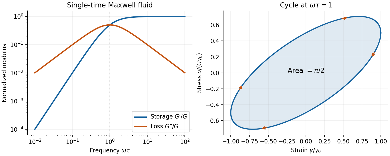
Original Maxwell storage and loss moduli, with a stress–strain cycle whose enclosed area measures dissipated work
. Details. 
Oscillatory rheometry measures stress amplitude and phase while imposing a small strain. An oscillatory-shear amplitude sweep first identifies a linear regime; an oscillatory-shear frequency sweep then measures and . Repeat at controlled temperature, suppress evaporation, check wall slip and sample aging, and correct instrument inertia at high frequency. Frequency-dependent structure and a nonlinear response cannot be inferred reliably by fitting one spring and dashpot to one point.
Articles by others on the same topic
There are currently no matching articles.