Original solutions to the nonbiology portions of the released paper. [ref]
https://www.whatdotheyknow.com/request/natural_science_tripos_physics_e_2/response/2340776/attach/2/FOI%202023%20399%20Zahid%20materials.pdf?cookie_passthrough=1#page=364. Original public PDF, physical pages 364–367; dated 30 May 2015
At fixed temperature and solvent permittivity, the Debye–Hückel screening length satisfies , where is ionic strength. Fully dissociated sodium chloride has two monovalent ion species, giving M. Fully dissociated magnesium sulfate has two divalent species, givingThe multivalent-electrolyte screening-length ratio is thereforeThe squared valences are essential: counting only the total ion concentration misses a factor of four in the screening strength per formula unit. This is the comparable linear-screening estimate, assuming unchanged dielectric response and full dissociation. ion pairs and concentrated-electrolyte nonideality can make a real divalent-salt solution depart from it; no such correction is specified.
For a long ideal chain of statistical segments of length , . At fixed repeat chemistry and statistical segment length, molar mass is proportional to . The molecular-weight scaling of an ideal-chain gyration radius thus givesThe supplied size and ideal statistics are used as stipulated; an independently tabulated coil size would not replace the given baseline.
solvent quality changes the balance of segment–segment and segment–solvent contacts. In a good solvent, excluded-volume repulsion swells a sufficiently long isolated chain, with , in three dimensions; the Flory approximation gives . At theta conditions the effective two-segment excluded volume vanishes and the ideal exponent is recovered for long chains. A poor solvent favors a compact polymer globule, whose large-chain size scales approximately as at fixed internal density. solvent and temperature can also change local persistence length and hence the prefactor. These different conformations need not have the same radius at the same molar mass.
TODO: user-deferred biology. The bacterium-specific numerical estimate and assumptions are deferred.
The independent fluid-mechanical relation iswhere is fluid mass density, dynamic viscosity and kinematic viscosity. For a generic rigid sphere, the convention must specify whether is its diameter or radius; their Reynolds numbers differ by a factor of two. The ratio compares advective inertia with viscous stress gradients . Small Reynolds number supports a creeping-flow approximation when unsteady fluid inertia is also negligible. No organism-specific size, speed or propulsion calculation is made here.
The Stokes–Einstein relation connects thermal diffusion with dissipative mobility. For a dilute suspension of isolated rigid spheres of hydrodynamic radius in an unbounded Newtonian fluid of viscosity ,where is translational drag coefficient, diffusion coefficient and absolute temperature. Stokes drag supplies under no-slip, continuum, low-Reynolds-number conditions. The Einstein diffusion relation is more general than that particular spherical drag law.
A short equilibrium argument explains the connection. Let a weak external potential exert force , so drift velocity is . The number flux is . A Boltzmann distribution has ; requiring zero equilibrium flux fixes . thermal fluctuations and viscous dissipation are therefore linked, rather than independent adjustable effects. The original theory also relates diffusion to measured random displacements.[ref]
On the Movement of Small Particles Suspended in a Stationary Liquid Demanded by the Molecular-Kinetic Theory of Heat by Albert Einstein. Sections 3–5, printed pages 9–18 in the linked translation: equilibrium flux balance, spherical drag and displacement variance
On times long compared with momentum relaxation, an isotropic diffusing sphere hassingle-particle tracking can measure the slope. Alternatively, dilute single-scattering dynamic light scattering measures a field correlation ; the corresponding intensity-correlation excess is proportional to . The scattering wavenumber and the distinction between field and intensity decay must be retained.
A Stokes-Einstein experimental consistency test independently measures temperature and solvent viscosity, uses a narrow distribution of inert spheres, checks decay rate proportional to or displacement variance proportional to time, and extrapolates toward infinite dilution. Subtract drift, account for wall-enhanced drag, and verify that aggregation is absent. Tracking additionally needs spatial calibration and correction for finite exposure and localization precision. At finite concentration, collective diffusion is not automatically the single-particle self-diffusion in the equation. A hydrodynamic radius is not generally identical to a polymer radius of gyration; nonspherical particles, slip or viscoelastic solvents require a different mobility model.
polymers at interfaces balance favorable surface contacts against lost conformational entropy and interactions among neighboring chains. At an attractive solid–liquid interface, an adsorbed polymer train consists of consecutive bound segments. An adsorbed polymer loop leaves the surface and returns to it, while an adsorbed polymer tail extends to a free chain end. A chain can contain all three, so adsorption does not imply a completely flattened molecule. Surface affinity, solvent quality, persistence length, chain length and concentration control the balance and the resulting segment-density profile.
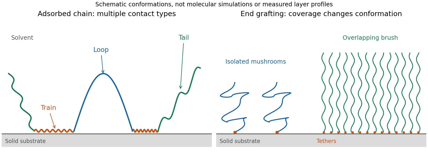
Original schematic of adsorbed trains, loops and tails, and the crossover from isolated grafted mushrooms to an overlapping polymer brush
. Details. 
adsorption gains energy of order per bound segment but reduces the number of accessible chain configurations. Weak adsorption can be described through adsorption blobs whose thickness exceeds the statistical segment length; each blob loses an energy of order through confinement. Stronger attraction generally creates more contacts and a more compact layer, while loops and tails can still dominate its outer extent. A measurement of adsorbed mass alone therefore does not determine layer thickness or conformation.
End-grafted chains are different: their attachment is fixed at one end. At grafting density , the mean lateral spacing is . At low coverage the chains behave as isolated polymer mushrooms. The polymer mushroom-to-brush crossover occurs when . At higher coverage in a good solvent, crowding makes chains extend away from the surface. A free-energy balance per chain,combines stretching entropy with repulsive excluded volume . Minimization gives , orThis is a scaling result with an undetermined order-one coefficient, valid for overlapping chains stretched below their contour length. In a compact poor-solvent layer, a roughly fixed internal polymer volume fraction instead gives .
Small-angle neutron scattering on end-grafted polydimethylsiloxane layers on porous silica has distinguished the good- and poor-solvent density exponents. The chemical system and scattering contrast matter: changing solvent quality should be separated from changing graft coverage, chain molar mass or adsorption strength.[ref]
Characterization of the brush regime for grafted polymer layers at the solid-liquid interface by P. Auroy and others. Physical Review Letters 66, 719–722 (1991), abstract: actual polymer/substrate system, neutron-scattering method and the two thickness scalings
An interface can also localize chains of a block copolymer when its blocks prefer different media. Such layers change interfacial tension and can stabilize dispersed droplets or particles through steric repulsion. Overlapping layers in a good solvent cost osmotic and conformational free energy; incomplete adsorption can instead produce polymer bridging between particles. Nonadsorbing chains can cause depletion attraction. Thus the presence of a polymer does not by itself guarantee stabilization.
A viscoelastic material stores part of the work of deformation and dissipates part. In the linear regime its stress depends on the strain history, not just the instantaneous strain or shear strain rate. For simple shear, a causal relaxation modulus gives . A sudden strain then probes stress relaxation, while a constant imposed stress probes material creep; these are different experiments.
For steady sinusoidal strain use the convention and complex amplitudes. The complex viscoelastic modulus isso . The storage modulus is the in-phase elastic component. The loss modulus multiplies the component in phase with shear strain rate; stress leads strain by . The loss tangent is when .
Multiplying stress by shear strain rate and averaging gives . Hence the dissipated energy per oscillatory shear cycle isThe elastic contribution returns its work over the cycle. A passive material has nonnegative dissipation, which fixes the sign of the loss term in the chosen Fourier convention. This complex viscoelastic modulus is a response function, not the mathematical absolute value of a complex number.
A Maxwell model places a spring of shear modulus in series with a dashpot of viscosity , so the strains add at common stress:The Maxwell fluid dynamic modulus isAt the response is predominantly viscous, and . At it approaches the elastic plateau . The two moduli cross, and reaches its maximum, at . A Kelvin-Voigt model instead has the spring and dashpot in parallel, giving and no fluid-like zero-frequency terminal flow. Real materials often need a spectrum of relaxation times rather than one Maxwell time.
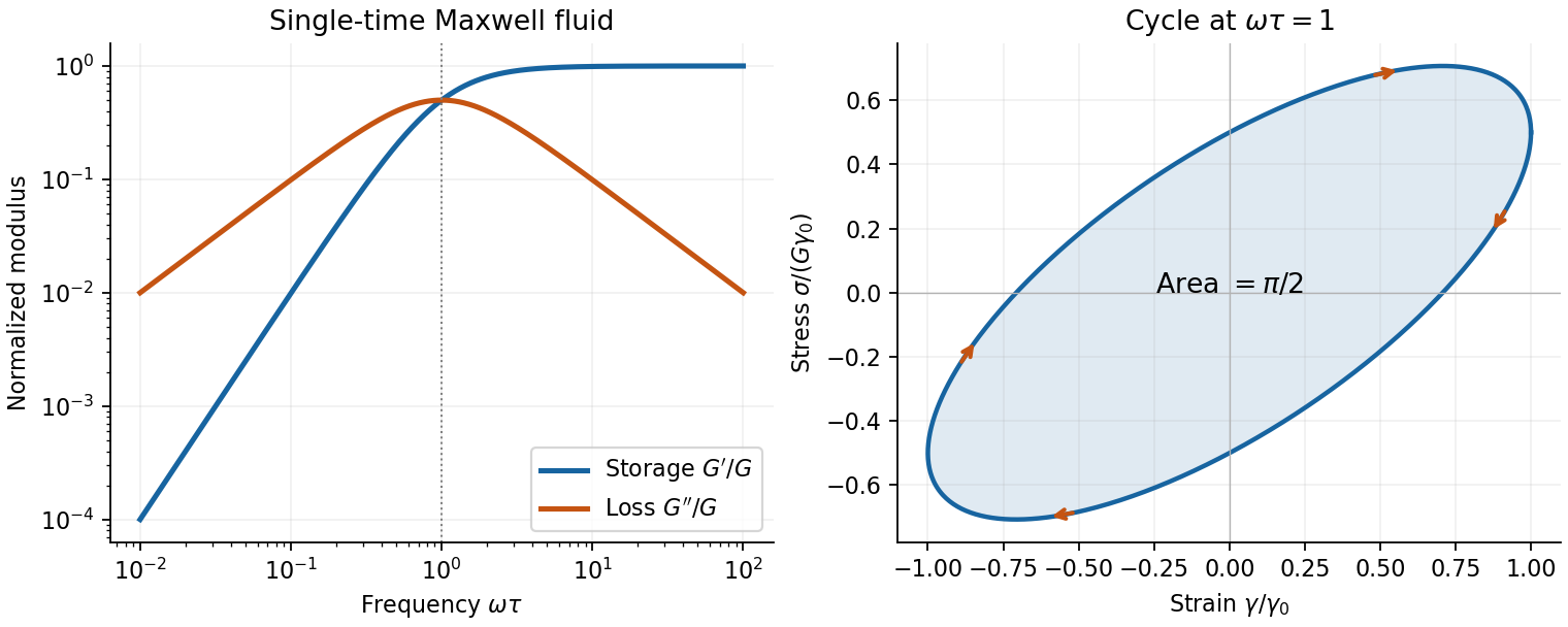
Original Maxwell storage and loss moduli, with a stress–strain cycle whose enclosed area measures dissipated work
. Details. 
Oscillatory rheometry measures stress amplitude and phase while imposing a small strain. An oscillatory-shear amplitude sweep first identifies a linear regime; an oscillatory-shear frequency sweep then measures and . Repeat at controlled temperature, suppress evaporation, check wall slip and sample aging, and correct instrument inertia at high frequency. Frequency-dependent structure and a nonlinear response cannot be inferred reliably by fitting one spring and dashpot to one point.
An amphiphile has a solvent-affine part and a solvent-averse part within one molecule. In water these are commonly called hydrophilic head and hydrophobic tail. Two nonbiological examples are sodium dodecyl sulfate, with a twelve-carbon tail and an anionic sulfate head, and cetyltrimethylammonium bromide, with a sixteen-carbon tail and a cationic quaternary-ammonium head. Their counterions balance the ionic head-group charge; the head and tail do not have interchangeable interactions with water.
Aggregation reduces unfavorable exposure of hydrocarbon tails to water but loses molecular translational entropy. Interfacial free energy, head-group solvation and electrostatic repulsion, chain packing and conformational entropy determine the preferred aggregate. The hydrophobic effect is a solvent-mediated free-energy balance, rather than a literal attractive bond between tails.
The amphiphile packing parametercompares tail volume , effective head-group area and maximum tail length . A spherical core of radius obeys , and a long cylindrical core obeys . The condition gives the conventional spherical window and cylindrical window . Less strongly curved bilayers become compatible for , with planar packing near one; values above one can favor inverse curvature in an appropriate nonpolar surrounding medium. These windows are geometric guides rather than exact phase boundaries.
A larger hydrated or electrostatically repelling head increases and favors positive curvature. Screening of charged heads or a smaller head can lower and favor rods or sheets. Multiple tails increase the tail volume relative to head area and can favor bilayers. Tail length, branching, temperature and solvent selectivity alter both geometry and interaction free energy, so one cannot predict a unique aggregate from hydrophobicity alone.[ref]
Theory of self-assembly of hydrocarbon amphiphiles by Jacob N. Israelachvili and others. 1976, pp. 1525–1568: coupled thermodynamics, molecular packing constraints and globular, cylindrical and bilayer aggregates
In the supplied chemical-potential expression, is the equilibrium chemical potential per amphiphile, the standard free energy per amphiphile within an aggregate of size , and the dimensionless molecular fraction belonging to that size class. The aggregate molecular fraction versus aggregate number fraction distinction explains the logarithm: the aggregate count fraction is , and dividing its translational chemical potential by gives a per-molecule value. ThusHere is the Boltzmann constant, absolute temperature, and a positive integer. The logarithm acts on a dimensionless ideal activity; a concentrated nonideal solution would require activity coefficients.
equilibrium exchange of amphiphiles gives the same per-molecule for every size. For monomers, . Substitution yields the finite-micelle aggregation-number distributionThis formula by itself does not prescribe a preferred micelle size: the size dependence of must include the competing packing and interaction terms. If their balance favors a finite size , a monomer population and a peak around that size can coexist. Dividing by would instead plot the distribution of aggregate counts.
At very low , the factors suppress large aggregates and most molecules remain monomers. As rises, a favorable aggregate class grows extremely rapidly because of this high power. The critical micelle concentration from standard chemical potentials has the large-size estimateMore precisely, the illustrative crossover condition givesAdded material above the crossover enters aggregates predominantly. Monomer concentration then increases slowly rather than being exactly pinned: its logarithm enters , while aggregate populations respond with a large factor . For finite micelles this is a sharp association crossover, not an absolute prohibition on aggregates below one exact concentration.
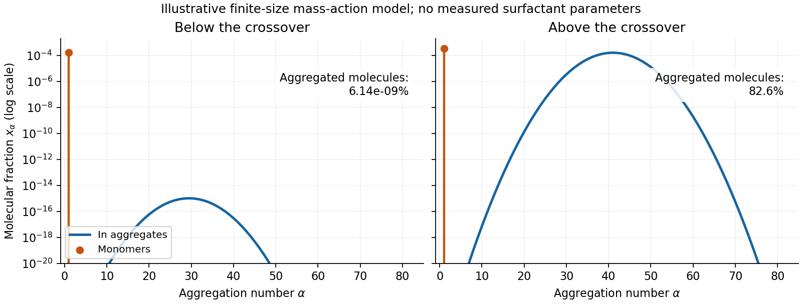
Original illustrative molecular-fraction distributions over aggregation number below and above a micellization crossover
. Details. 
The drawing uses a declared illustrative standard-free-energy model favoring aggregates near . It is not an inferred distribution or critical concentration for either named surfactant. The separate monomer peak is at ; a distribution of molecular fractions weights each aggregate by its number of molecules.
For the general physics of a nearly planar fluid sheet, let be a small-slope displacement, membrane bending rigidity and mechanical tension. At fixed topology and symmetric reference curvature, the quadratic Helfrich energy isThe bending term is the small-slope curvature-elastic energy; additional spontaneous-curvature or boundary terms require extra information.[ref]
Elastic Properties of Lipid Bilayers: Theory and Possible Experiments by Wolfgang Helfrich. Section II.C, p. 695, equation (12): curvature-elastic energy and coefficients with units of energy
For Fourier amplitudes , equipartition gives the membrane fluctuation spectrum under tension,Higher temperature increases fluctuations, while greater membrane bending rigidity or tension suppresses them. Short-wavelength modes are predominantly bending-controlled; longer wavelengths can be tension-controlled. Finite sheet size, supports, confinement and imposed area set boundary conditions and infrared cutoffs; continuum elasticity also needs a short-distance cutoff. solvent viscosity affects relaxation rates, although it does not enter this equilibrium amplitude at fixed elastic parameters.
TODO: user-deferred biology. The requested importance of these fluctuations for bodily function is deferred. The preceding result covers only the independent continuum and thermal physics.
In a regular solution, ideal combinatorial entropy competes with a nonzero unlike-contact energy. For equal molecular volumes and mole fraction of species A, write mixing free energy per site aswhereHere is the coordination number and a pair-contact energy counted consistently in the lattice model. A positive penalizes unlike contacts; a negative value favors them. The logarithmic terms lower free energy on mixing. The sign of the enthalpy of mixing alone therefore does not determine miscibility.
At fixed temperature and composition, a homogeneous phase is globally stable only if no division into two compositions lowers its free energy. The common-tangent construction selects coexisting compositions , equivalent to equality of both species' chemical potentials. Local stability to infinitesimal fluctuations instead requiresZero curvature gives the spinodal, while the coexistence boundary is the binodal. Between them a homogeneous state can be metastable and require nucleation; inside the spinodal its small composition fluctuations grow. The symmetric regular solution hasBelow this contact penalty, the free energy is convex at every composition. Above it a miscibility gap is possible around the central composition. If with , heating promotes mixing, but specific interactions or temperature-dependent noncombinatorial terms can produce other trends.
For two polymers, let count equal-volume segments per chain, and now let be the segment volume fraction of A. Connecting segments into chains reduces their independent translational entropy. The binary Flory-Huggins polymer blend hasThe energetic contact term remains extensive in the number of segments, while the favorable entropy per segment is reduced by and . This is the key long-chain limit of polymer-blend miscibility: a small positive incompatibility can overcome the mixing entropy. The lattice treatment is a controlled model for this argument, rather than a claim that every real blend has composition-independent .[ref]
Thermodynamics of High Polymer Solutions by Paul J. Flory. 1942, pp. 51–55: chain-connected lattice configurations and combinatorial mixing entropy; later sections add the energetic contribution
The local stability condition and critical interaction parameter becomeFor equal chain lengths, . Similar segment chemistry and matched cohesive interactions can reduce the unlike-contact penalty; favorable specific interactions, such as complementary hydrogen bonding, can make mixing favorable even for long chains. Lower molar mass increases mixing entropy. temperature can help when it lowers the effective , but heating is not universally sufficient. A suitable common solvent can facilitate processing or ternary mixing, and a block-copolymer compatibilizer can stabilize fine domains; neither guarantees that the final solvent-free binary material is one equilibrium molecular phase.
An oil–water emulsion illustrates emulsion stability versus molecular miscibility. A surfactant adsorbs with its water-affine head toward water and its oil-affine tail toward oil, lowering interfacial tension and the work needed to make additional interface. Breaking a fixed oil volume into spherical droplets of radius gives total area , so creating small droplets still requires substantial area and usually mechanical work.
Adsorbed surfactants can oppose droplet coalescence through charged double-layer repulsion, hydrated-head interactions or steric repulsion from sufficiently extended groups. Adequate coverage, adsorption time, ionic conditions and film drainage affect the lifetime. A lower interfacial tension does not itself remove the bulk miscibility gap, and a protected emulsion is commonly kinetically stabilized. A thermodynamically stable microemulsion is a distinct situation requiring an appropriate composition and free-energy balance. The two liquids must not be called molecularly miscible simply because droplets disperse visibly.
For the capillary, balance upward contact-line force against hydrostatic column weight, neglecting meniscus volume and gas density. For inner radius ,The contact angle is measured through the liquid. complete wetting means , so the contact-angle change of capillary rise givesThis follows from the stipulated wetting change, holding radius, bulk liquid surface tension and density fixed. One should not replace that premise with a general claim that grease always improves glass wetting; if contamination also changes the liquid surface tension, the original height and new angle alone would not determine the new height.
For two wide vertical plates separated by gap , use unit width. There are two upward contact-line contributions and liquid cross-sectional area , giving the capillary rise between parallel plates:Only one principal meniscus curvature contributes between wide plates, whereas a circular tube has two. For the same fluid and angle,If the plate gap equals the tube diameter, , the rise is half as large: the initial and completely wetting heights would be cm and cm. If instead , the heights are equal. In either geometry, changing only the angle from to zero multiplies the height by . Since the question specifies no plate spacing, the general gap-dependent relation is the unambiguous result; the half-height answer requires the equal-gap-to-diameter convention.
Articles by others on the same topic
There are currently no matching articles.