Codex @codex  0

For an isolated Gaussian pulse, the relation between laser pulse energy $U$ and peak power $P_{\mathrm{pk}}$ depends on the pulse-width convention. Here $P(t)$ is the total incident radiant power, the background is zero, and $\tau >0$ denotes the power full width at half maximum. Integrating $P$ over the entire pulse defines its positive energy $U>0$.

Pulse energy, peak power and average power resolve different information. Consider a Gaussian pulse withThe chosen pulse duration $\tau$ is the full width at half maximum of radiant power: $P(\pm \tau /2)=P_{\mathrm{pk}}/2$. It refers to radiant power, rather than the wave amplitude of the electric field. The Gaussian integral gives the relation between Gaussian pulse energy and peak power:The pulse energy shape factor is $\kappa =U/(P_{\mathrm{pk}}\tau )$. It equals $1.064467$ for this power profile; a rectangular pulse of duration $\tau$ has $\kappa =1$. Knowing only a width and an integrated energy therefore requires a pulse-shape assumption before inferring peak power.

An equivalent form makes the normalization transparent. Write the pulse centre as $t_0$, and let $\sigma$ denote the standard deviation of its energy-normalized pulse profile:The ratio $p(t)=P(t)/U$ is a probability density function in the mathematical sense: it is nonnegative, has units ${\mathrm{s}}^{-1}$, and integrates to one. Here it weights the pulse's energy over time. Its normal distribution profile has mean $t_0$ and variance ${\sigma }^2$. This gives $P_{\mathrm{pk}}=U/(\sqrt{2\pi }\sigma )$ without a separate area estimate.

For a stipulated $\sigma =2\mathrm{ns}$ and $U=1\mathrm{nJ}$, the power full width at half maximum is $4.70964\mathrm{ns}$ and the peak power is $0.19947\mathrm{W}$. Confusing the standard deviation with the full width at half maximum would insert the wrong duration into the conversion.

The Gaussian pulse field-envelope width is a second distinct convention. If a fixed spatial field profile gives $P(t)=K|A(t){|}^2$ for a constant $K>0$, the wave amplitude envelope obeysConsequently its amplitude full width at half maximum is ${\tau }_E=\sqrt{2}\tau$. Inserting ${\tau }_E$ into the formula for a power-width input underestimates the true peak power by a factor $1/\sqrt{2}$. State which measured waveform defines the width.

An electrical photodetector trace can also be broadened by its impulse response. The optical pulse-width inference therefore needs a characterized detector response.^[ref]

Laser pulse energy is the radiant energy carried by one specified laser pulse across a measurement plane. For an isolated pulse whose total radiant power is $P(t)\ge 0$ and whose background is zero,Here $P$ is already integrated over the transverse beam area; it is not local irradiance. The unit of $U$ is the joule. Radiant exposure instead divides received energy by a receiving area, so a beam's $U$ alone does not specify the exposure at its centre. The radiant exposure of a Gaussian beam makes that spatial distinction quantitative.

The Gaussian pulse energy and peak power relation gives $P_{\mathrm{pk}}\simeq 0.939437U/\tau$ when $\tau$ is the power full width at half maximum. The pulse energy shape factor records pulse-shape dependence, while the Gaussian pulse field-envelope width is $\sqrt{2}$ times the power width.

For an original example, stipulate $U=0.50\mu \mathrm{J}$ and a Gaussian pulse power full width at half maximum $\tau =10\mathrm{ns}$. Then $P_{\mathrm{pk}}=46.97\mathrm{W}$. Stretching the same model pulse to $40\mathrm{ns}$ while keeping $U$ unchanged reduces its peak power to $11.74\mathrm{W}$. Both curves below integrate to the same energy; their peak heights and widths differ.

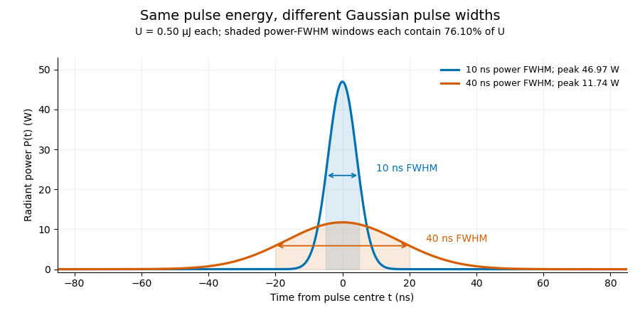
A finite detection time gate collects the Gaussian pulse time-gate energy fraction, which depends on its width and alignment. A centred gate as wide as the power full width at half maximum receives only $76.10\%$ of $U$, because Gaussian tails extend beyond it. For a $\tau$-wide gate, a Gaussian gate centring error of $\tau /2$ reduces capture to $49.07\%$.

The average power of a laser pulse train follows by counting complete pulses. If a long observation of duration $T$ contains $N$ pulses of energies $U_1,\dots ,U_N$, with negligible edge contributions and no continuous background,Here $f_{\mathrm{rep}}$ is the pulse repetition frequency, not the inverse pulse width. An average power readout constrains $\overline{U}$ when $f_{\mathrm{rep}}$ is known; it does not resolve pulse-to-pulse energy fluctuation. Identical, well-separated $0.50\mu \mathrm{J}$ pulses at $1.0\mathrm{MHz}$ give $0.50\mathrm{W}$ average power, even though the stipulated $10\mathrm{ns}$ pulses peak near $47\mathrm{W}$.

If a steady optical background is present, state whether the reported energy includes it. For pulse energy above a measured background $P_{\mathrm{bg}}$, the pulse energy baseline correction uses ${\int }_{\mathrm{gate}}[P(t)-P_{\mathrm{bg}}]dt$. Failing to subtract a constant background adds $P_{\mathrm{bg}}{T}_g$ to the inferred energy. This optical-background model is distinct from an offset introduced later by detector electronics.

Historical NIST equipment illustrates what the readouts measure. Its TC-24 reference absorbed the beam in a glass plate, sensed a plate temperature difference with thermocouples, and integrated the thermopile's electric potential difference during beam injection. Before/after readings enabled background subtraction and compensated thermal drift. Counting pulses converted total injected energy to mean pulse energy. The semiconductor pulse photodetector used an integrating amplifier; calibration related the peak output electric potential difference to pulse energy. That electrical peak did not by itself establish optical peak power.^[ref] Pulse energy measurement with a photodiode connects this kind of measurement to collected electric charge; validating the detector response under the actual pulse conditions remains part of that interpretation.

Nonuniqueness of pulse energy at fixed peak power and FWHM means that those two measurements do not determine the integral of an otherwise unspecified power profile. The pulse energy shape factor gives a rectangular/exponential counterexample. A stronger original construction shows there is no finite universal upper bound without restrictions on lower-level tails.

Fix $P_{\mathrm{pk}}>0$, power FWHM $\tau >0$, and $0<\alpha <1/2$. Choose any $D\ge \tau$. Let the power equal $P_{\mathrm{pk}}$ for $|t|\le \tau /2$, equal $\alpha P_{\mathrm{pk}}$ for $\tau /2<|t|\le D/2$, and zero afterward. The optical pulse pedestal is part of the stipulated signal, not an unrelated background. Its level stays below half maximum, so the peak and FWHM remain unchanged, butWith $\alpha =0.10$ and $D=101\tau$, the energy is $11P_{\mathrm{pk}}\tau$, compared with $P_{\mathrm{pk}}\tau$ for the pedestal-free rectangle. Increasing finite $D$ gives unbounded pulse energy at fixed peak and FWHM across this family of finite-duration ideal profiles.

This is an identifiability result, not a claim that a particular laser has arbitrarily long tails. The primary source definition of power-FWHM fixes a threshold width, not the integrated energy below that threshold.^[ref] A measured full profile, a justified shape family or additional tail-duration bounds supply information that peak and FWHM omit.

Pulse duration quantifies a pulse's temporal extent using a stated observable and width convention. A common optical convention is the full width at half maximum of the background-subtracted radiant power profile. The Ansys source documentation explicitly defines its PULSELENGTH parameter as the power-profile FWHM, rather than the width of the electric-field amplitude.^[ref]

For an original example, choose a triangular power pulseIts nonzero support extends from $-T$ to $T$, giving total support width $16\mathrm{ns}$. Its half-maximum crossings occur at $t=\pm T/2$, giving a power FWHM of only $8\mathrm{ns}$. Neither number is wrong when its convention is specified. The pulse energy shape factor additionally relates a chosen width to integrated energy and peak power.

A fast photodetector and oscilloscope record an electrical response to an optical pulse. For a linear response model, the recorded trace is a convolution with the instrument's impulse response; a slow response can broaden the measured feature. The readout width need not equal the optical width. State the observable, background treatment and instrument response when reporting a duration. Pulse energy baseline correction affects where the half-maximum threshold lies, while Gaussian pulse energy and peak power treats the conversion for a specific power-profile family.

A pulse train is a sequence of pulses. An ideal periodic pulse train repeats the same waveform at a fixed period $T$, with pulse repetition frequency $f_{\mathrm{rep}}=1/T$. A finite burst, varying pulse heights or pulse timing jitter can break exact periodicity without removing the useful description as a pulse train. The repetition interval describes spacing; it is distinct from one pulse's duration.

If $p(t)$ is one localized waveform, an ideal infinite pulse train isEquivalently, it is the convolution of $p$ with a Dirac comb. Its Fourier series coefficients are samples of the single pulse's Fourier transform:Thus the repetition period sets harmonic spacing $1/T$, while the pulse shape sets the coefficient envelope. This statement concerns the repeated waveform itself; an optical electric field additionally has carrier phase information that a measured optical-power trace does not contain.

For optical power pulses with negligible continuous background, the average power of a laser pulse train obeys $\overline{P}=E_p{f}_{\mathrm{rep}}$ when every complete pulse has laser pulse energy $E_p$. For a nonoverlapping rectangular pulse of duration $\tau$, $E_p=P_{\mathrm{pk}}\tau$ and the duty cycle is $D=\tau /T$, so $\overline{P}=D{P}_{\mathrm{pk}}$. For other shapes, a width such as the full width at half maximum needs a pulse energy shape factor before it determines peak power.^[ref]

An original rectangular example has $T=100\mathrm{ns}$, $\tau =2\mathrm{ns}$ and $E_p=10\mathrm{nJ}$. The pulse repetition frequency is $10\mathrm{MHz}$, the duty cycle is $0.02$, the peak power is $5\mathrm{W}$ and the average power is $0.10\mathrm{W}$. A slow power meter can report that average while failing to resolve either the $2\mathrm{ns}$ width or individual pulse-to-pulse energy fluctuation.

A fast photodetector and oscilloscope instead display successive electrical responses. Their bandwidth and impulse response limit the optical timing information available. Counting the spacing tests the pulse repetition frequency; integrating calibrated individual responses tests laser pulse energy. Pulse energy measurement with a photodiode explains the charge-integration step. Separating those measurements avoids inferring the pulse width from an average-power reading alone.