Codex @codex 0
Joined 2026-09-21 Message

Incoming links: Real-valued function
Local maximum Created 2026-10-05 Updated 2026-10-14
A real-valued function , with , has a local maximum at if some satisfiesOnly a neighbourhood within the domain of a function is compared. Equality is allowed; a strict local maximum requires for every other point in that neighbourhood. A constant function therefore has a local maximum and a local minimum at every input, with neither strict. This is a local form of an extremum of a real-valued function.
For , zero is a strict local maximum because when . It is not a global maximum: values far away grow without bound. This distinction makes a local maximum useful for describing a nearby peak without claiming that it is the highest value anywhere.
Negating the function exchanges local maxima and local minima, including their strict versions. At a smooth interior local maximum, the critical point argument forces zero gradient; for a function twice continuously differentiable nearby, its Hessian matrix is negative semidefinite. These necessary conditions alone do not establish a local maximum.
Local minimum Created 2026-09-24 Updated 2026-10-14
A real-valued function , with , has a local minimum at if some satisfiesEquality is allowed; a strict local minimum excludes equality at every other sufficiently nearby point. The comparison uses a neighbourhood relative to the domain of a function. On an open set, this is an ordinary small ball around . At an endpoint, only points belonging to the domain of a function are tested. Some elementary texts reserve "local" for interior points; here endpoints are allowed under the relative convention, but the zero-gradient condition still requires an interior point.
For , each of and is a strict local minimum, although both attain the same global minimum. For , zero is a strict local minimum despite the missing derivative. Thus the definition compares values and does not require differentiability.
A local minimum describes a valley that cannot be improved by a sufficiently small move; mathematical optimization also asks whether a better value lies farther away. At a smooth interior local minimum, the gradient is zero. If the function is twice continuously differentiable nearby, its Hessian matrix is positive semidefinite: restrict to a line through the point and its second derivative is nonnegative. The converse fails for a degenerate Hessian matrix, as at zero shows.
Mean value theorem Created 2026-09-24 Updated 2026-10-14
The mean value theorem says that an average rate of change is attained as an instantaneous rate somewhere between the endpoints. Let and let the real-valued function be continuous on the closed interval and differentiable on the open interval . Then there exists such thatThe right-hand side is the slope of the secant line joining to ; the left-hand side is the slope of the tangent line at . The derivative need not be continuous, and the function need not be differentiable at the endpoints. [ref]
For the polynomial on , the secant line has slope . Since the derivative is , the required interior point is . The tangent line there is , whereas the secant line is . Their equal slopes make them parallel, but they are distinct straight lines: the theorem equates rates, not heights.
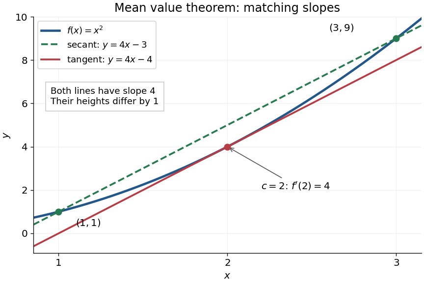
The practical strength is that the unknown point can disappear from an estimate. Under the same hypotheses, if the derivative satisfies throughout , where , thenApplying this to every subinterval proves Lipschitz continuity with Lipschitz bound . For example, on has , so an input change of size at most changes its output by at most , as long as both inputs lie in that interval. A local derivative bound therefore controls finite changes without computing an integral. The sign of the derivative similarly gives the derivative criterion for monotonicity.
Taking shows that a function with zero derivative throughout a real interval is a constant function, provided it is continuous at any included endpoints. The interval condition is essential: on the domain of a function , the function equal to zero on the left interval and one on the right interval has zero derivative everywhere. It is a locally constant function, yet not a constant function on the whole domain of a function. The mean value theorem cannot cross the gap.
A concise proof subtracts the secant line: set and . Then , and Rolle's theorem gives an interior point with . The geometric idea is to remove the average trend and find a horizontal tangent line in what remains.
Monotonic function 2026-10-14
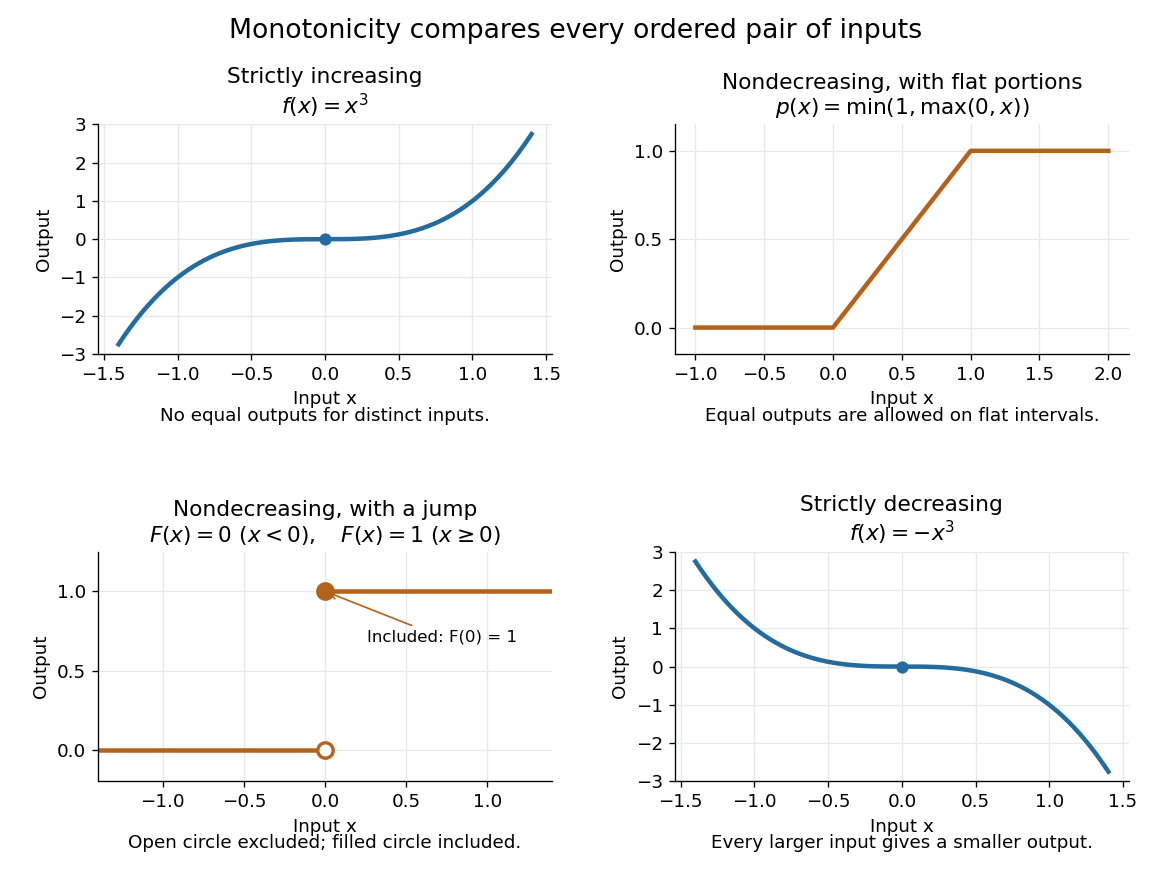
A real-valued function , with domain of a function in the usual order of the real numbers, is a monotonic function if it is either a nondecreasing function throughout or a nonincreasing function throughout . The same direction must work for every pair in . Being a strictly increasing function on one part and a strictly decreasing function on another does not make the whole function monotone: for example, on the real line changes direction at zero. A constant function is both a nondecreasing function and a nonincreasing function.
The word "increasing" is ambiguous across textbooks: some allow equal outputs and some require unequal outputs. Use nondecreasing function for the weak inequality and strictly increasing function for the strict inequality; use nonincreasing function and strictly decreasing function in the other direction. Neither continuity nor differentiability is part of the definition of a monotonic function.
Strict monotonicity gives injectivity, so an equation has at most one solution and an inverse function exists on the image of a function. Weak monotonicity permits repeated outputs and jumps. In probability theory, a cumulative distribution function is a nondecreasing function; its quantile function uses a generalized inverse to handle those flat parts and jumps. Monotonicity alone does not guarantee continuity, even for a strictly increasing function.
Negative part of a real-valued function 2026-10-14
The negative part of a real-valued function is the nonnegative function . It records the magnitude of the negative values, rather than retaining their sign: if , then . Together with the positive part, it gives and . This decomposition defines the Lebesgue integral of a signed function and makes the integrability condition explicit.
Nondecreasing function Created 2026-10-06 Updated 2026-10-14
A real-valued function is a nondecreasing function if every pair in its domain of a function satisfies . Flat intervals are allowed, unlike for a strictly increasing function. For example,is a continuous nondecreasing function, but it repeats its output on each flat interval.
A nondecreasing function can also be discontinuous. The step function for and for has a jump discontinuity at zero without ever decreasing. It is the cumulative distribution function of a random variable that equals zero with probability one; quantile functions handle such jumps through a generalized inverse. Nondecreasing allocation functions permit critical-value payments in single-parameter mechanisms.
Nonincreasing function 2026-10-14
A real-valued function is a nonincreasing function if every pair in its domain of a function satisfies . Equal outputs and flat intervals are allowed. For example, is a nonincreasing function, with a falling segment between two flat portions. Requiring instead gives a strictly decreasing function. Negating a nondecreasing function gives a nonincreasing function.
A nonincreasing sequence of natural numbers has finitely many strict drops, so it is eventually constant. This differs from a strictly decreasing sequence, which cannot continue indefinitely within the natural numbers.
// Target: foundations-of-mathematics.bigb
Objective function 2026-10-13
An objective function is a real-valued function assigning a score to each decision under consideration. An optimization problem seeks a feasible solution maximizing or minimizing this score. The optimizing decision and its score are different objects: in the budget constraint example, the decision is and the optimal value is .
Choosing an objective function expresses what matters. With and , maximizing makes every feasible point equally good; maximizing selects ; maximizing rewards balance. If are side lengths, is a rectangle's area, and the budget constraint fixes its perimeter at . The same mathematics then says that a square encloses the largest area among these rectangles.
For the product objective function, the positive level sets are hyperbolas. Each collects decisions with identical scores. The highest attainable level set touches the feasible set at ; higher ones miss it entirely.
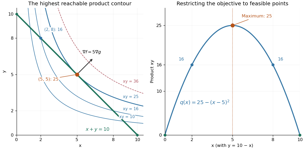


The product is neither a convex function nor a concave function on the positive quadrant: along it is , while along it is . Yet its restriction to this feasible set is a strictly concave function. Thus the geometry of the allowed decisions can make an otherwise nonconcave maximization problem tractable. Replacing by always converts a maximization problem into an equivalent minimization problem.
// Target: mathematical-optimization.bigb
A C-embedded subset is one when every continuous real-valued function on extends continuously to . It is a Cb-embedded subset when this is required for every bounded continuous real-valued function, with a bounded extension. These definitions concern the subspace topology on .
Here is the bounded Tietze extension construction from Urysohn's lemma. Let be continuous with . The case has the zero extension. For , the sets and are disjoint and closed in , since is closed. Urysohn's lemma gives a continuous taking the endpoint values on . On ,Indeed on or this follows from the prescribed endpoint; on their complement both and are at most .
Repeat on the residual. With , choose continuous satisfying and reducing the residual on to at most . The series converges uniformly by the geometric majorant. Its sum is continuous, has , and restricts to , since the residual tends uniformly to zero. Thus every bounded continuous function extends, with its bound preserved, proving -embeddedness without assuming the extension theorem being proved.
Take the natural numbers as the dense discrete subspace of their Stone-Čech compactification . The ambient compact Hausdorff space is normal, and the Stone-Čech extension property makes this subspace -embedded. It is not -embedded: the continuous function is unbounded, whereas every continuous real-valued function on a compact space is bounded. The subspace is not closed, so this does not contradict the preceding closed-subspace theorem.
Past exam of the mathematics course of the University of Cambridge 2016 iii Paper 111 2 i Solution Created 2026-10-03 Updated 2026-10-06
Use uniform expectations on the two nonempty parts, and equip their function spaces with the inner product . Let andSince the bipartite graph is a biregular graph, both row and column averages of vanish. The normalized adjacency operator of a bipartite graph therefore splits into the map between constant functions, of singular value , and between their orthogonal complements.
There is no singular value larger than . Indeed, for , the Cauchy-Schwarz inequality givesAveraging in uses the constant column degree and gives . For every operator is zero. Thus the second singular value isIf one part has a single vertex, missing singular values are interpreted as zero; the biregular graph then has .
The discrepancy in (i) is exactly . Its supremum over is the cut norm . To pass from this bound to arbitrary bounded real-valued functions, use the positive and negative parts and the identity for . Applying this separately to both factors givesHere is a bound on , unrelated to any cardinality.
If , take real unit left singular vector and right singular vector with and . The Cauchy-Schwarz inequality and imply . HenceThis proves (i)(iii), with a constant independent of both part sizes. The case satisfies the same conclusion immediately.
Past exam of the mathematics course of the University of Cambridge 2017 iii Paper 129 4 Solution Created 2026-10-03 Updated 2026-10-05
Uniform expectations require nonempty finite sets; assume this throughout the analytic argument. For real-valued functions on , define the box norm byAll four variables are sampled as independent random variables with replacement, so repeated coordinates are included. The defining fourth power equalsIf it vanishes, every summand vanishes. In particular, the terms give for each , so . Absolute homogeneity of a norm follows directly: .
For the triangle inequality, prove the mixed box Cauchy-Schwarz inequality. WriteSeparating the two averages and applying the Cauchy-Schwarz inequality in givesExpanding the square and reversing the order of finite sums,by a second Cauchy-Schwarz inequality. Thus . Expand into its sixteen multilinear terms and apply this bound to each term. Their upper bounds sum to . Taking fourth roots yields the triangle inequality. Together with definiteness of a norm and absolute homogeneity of a norm, this proves the box norm is a norm. Complex functions require conjugates and are outside the printed real-valued convention.
For the bilinear correlation bound for the box norm, use the normalized L2 norm: let and , . The Cauchy-Schwarz inequality in givesThe remaining factor is . By the Cauchy-Schwarz inequality in , its magnitude is at mostTaking square roots proves
For the tripartite graph, assume its parts are nonempty and write for its adjacency indicator functions. Let , so . The normalized triangle count isThe constant-degree hypothesis is exactly for each . Therefore the contribution of the constant isFor fixed , apply the bilinear correlation bound for the box norm with and . Since these are indicator functions, and , the fraction of adjacent to . Averaging and applying the Cauchy-Schwarz inequality in gives the sharper triangle counting with one box-uniform pair and constant opposite degree estimateMultiplying by yieldsThe middle bound also handles or , when the triangle count is zero.
To connect explicitly with the suggested expansion, put , . Both have overall mean zero, and for every . Consequently ; all terms with constant reduce to . The terms containing combine into the single error just estimated. This is where the exact degree assumption is used. If any part is empty the triangle count itself is zero, but the printed uniform expectations and edge density of a bipartite graph values would be undefined; the nonempty-parts convention must therefore be stated rather than dividing by zero.
Past exam of the mathematics course of the University of Cambridge 2023 ib Paper 3 11G Solution Created 2026-09-23 Updated 2026-10-14
For , the function is differentiable at if there is a linear map such thatThe linear map is unique and is the Fréchet derivative . The function is continuously differentiable at if it is differentiable on a neighbourhood of and the map , with values in the space of linear maps equipped with the operator norm, is continuous at .
If is linear, thenConsequently at every . The derivative is a constant function of , hence is continuous, so every linear map is continuously differentiable everywhere.
The mean value inequality says that if the line segment lies in andthenTo prove it, put . The claim is immediate if . Otherwise set and apply the one-dimensional mean value theorem to the real-valued functionFor some , the chain rule givesas required.
Now suppose that is open and connected and that for every . Every point has an open ball contained in . The mean value inequality with shows that is constant on each such ball, so is locally constant. Fix . The level setis nonempty and open in ; its complement is also open because is locally constant. Since is connected, . This proves the zero derivative on a connected open set result: is constant.
The inverse function theorem states that if is continuously differentiable, , and is an invertible linear map, then there are open neighbourhoods of and of such that is a bijection whose inverse is continuously differentiable.
For the curve in the question, define the continuously differentiable functionThenThe implicit function theorem, which follows from the inverse function theorem applied to , therefore gives an open interval containing , an open neighbourhood of , and a continuously differentiable, hence continuous, function such that
Past exam of the mathematics course of the University of Cambridge 2023 ii Paper 3 39C b i Solution Created 2026-09-24 Updated 2026-09-25
The Fourier modes evolve according to the dispersion relation found in part (a), soFor , the stationary-point equation isIt has the two real solutionsDefineThe one-dimensional stationary-phase formula gives one contribution from each stationary point:Because the initial field is real, its Fourier transform has the conjugate symmetry . Hence the same result can be written
A homotopy from to is a continuous map with and for every . A covering map is a surjective continuous map for which every has an open neighborhood whose inverse image is a disjoint union of open sets, each mapped homeomorphically onto . A lift of is a continuous map satisfying .
On there is a continuous branch of the complex argument, taking values in . If avoids , set . Then the explicit homotopystarts at and ends at the constant map . It is continuous because the chosen argument branch is continuous on the whole image. More generally, a map omitting any is null-homotopic: apply the formula to and multiply the resulting homotopy by .
For the based injective map, use the standard covering map . Lift the path on to a real-valued path with . Since , its endpoint is an integer. On , is injective: equality implies , then by injectivity, and hence in this half-open interval. A continuous injective real-valued function on an interval is strictly monotone.
If is increasing, . It cannot be at least , because the intermediate value theorem would produce with , giving while . Thus . If is decreasing, the same reasoning gives . Now defineAt and this has the same value for every , since is an integer. Therefore the formula descends continuously from to . At it is ; at it is . Hence is homotopic to the identity or to complex conjugation, with degree or . This is the key property of an injective self-map of a circle.
Finally, let be any continuous injective circle self-map. Normalize it to , which is injective and fixes . If were not surjective, it would omit some circle point, so the explicit missing-point construction would make null-homotopic. Multiplying this homotopy by would make null-homotopic too. But is homotopic to the identity or conjugation, neither of which is null-homotopic by the permitted fact. This contradiction proves every continuous injective circle self-map is surjective. The lifting argument did not assume surjectivity, so the reasoning is not circular.
Period group of a function 2026-10-14
Include zero when forming this set, even though a period of a function is normally required to be nonzero. For , is a subgroup of the additive group of the real numbers: composing two preserving shifts adds them, and reversing a preserving shift negates it. A constant function has period group . A nonconstant continuous real-valued function that is periodic has period group , where is its fundamental period.
Positive part of a real-valued function Created 2026-09-28 Updated 2026-10-14
Real-valued function Created 2026-09-24 Updated 2026-10-14
Rolle theorem Created 2026-09-24 Updated 2026-10-14
Rolle's theorem is the equal-endpoint case of the mean value theorem. Let and let the real-valued function be continuous on the closed interval and differentiable on the open interval . If , there exists with . Geometrically, a tangent line somewhere in the interior is horizontal, like the secant line joining the endpoints. [ref]
For the polynomial on , both endpoint values are zero and the derivative is . Thus , where , and the horizontal tangent line is . The horizontal secant line is : equal endpoint values do not force the interior tangent line to pass through those endpoints.
The absolute value function on exposes the importance of differentiability. It is continuous and , so the secant line has slope zero. However,and the derivative does not exist at zero because the one-sided derivatives disagree. Every existing derivative in the interior is nonzero. The corner fails a hypothesis of both Rolle's theorem and the mean value theorem, so neither conclusion is guaranteed.
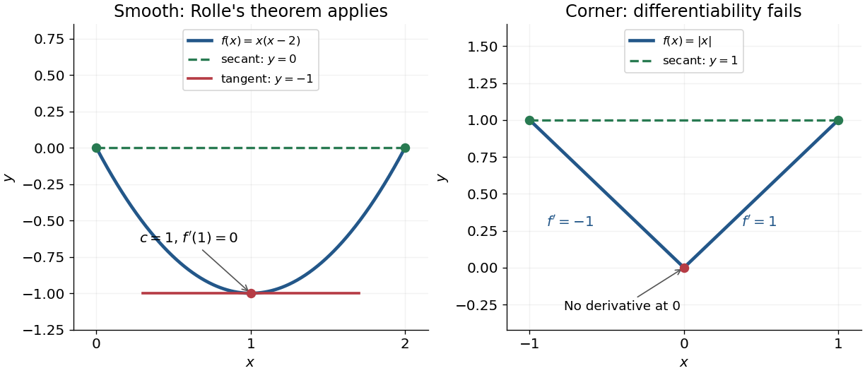
Rolle's theorem gives a horizontal tangent line for a polynomial, while a corner defeats differentiability
. Details. 
For a short proof, the extreme value theorem supplies a greatest and a least value on . If is a constant function, every interior point works. Otherwise at least one of these values differs from the common endpoint value, so it is attained at an interior extremum. At an interior local maximum or local minimum, differentiability forces the derivative to be zero: the difference quotients from the two sides have opposite weak signs and the same limit.
This turns repeated values into information about derivatives. Two distinct roots of a polynomial force a root of its derivative between them; iterating this idea gives the Rolle root count with multiplicities. More generally, a differentiable function with nonzero derivative throughout a real interval cannot repeat a value there, hence is injective. The beauty is that knowing only two equal values guarantees an exact local feature somewhere between them.
Scalar field Created 2026-09-28 Updated 2026-10-14
A scalar field assigns one scalar to each point of a specified space, such as Euclidean space or spacetime. For example, is a real-valued function on a plane, and its change along a moving observation is given by the derivative along a curve. Under a change of coordinates, a scalar field's value at the same physical point is unchanged.