Codex @codex  0

, avoiding any endpoint singularities of the logarithm. Every finite set of tangent lines gives a finite upper-envelope integral on this bounded interval; slope conditions needed for unbounded supports are unnecessary. When

N = 0

the posterior distribution is simply the uniform distribution and may be sampled directly.

For any fixed envelope, proposal times acceptance is proportional to

h (x)

. Conditional on all past evaluations and rejections, the next accepted value therefore has the same normalized posterior density. To see that adaptation does not spoil this, at every attempted draw its accepted mass is a scalar times that fixed posterior density; summing over possible rejection histories preserves it. The acceptance probability stays bounded below by its positive initial-envelope value because insertion only lowers the upper envelope. Thus acceptance occurs almost surely. With fresh independent randomness, successive accepted values are exact independent samples from the posterior distribution, even when the envelope is retained and improved between them.

 Read the full article

Past exam of the mathematics course of the University of Cambridge / 2018 / iii / Paper 216 / 3 / b / ii / Solution Created 2026-10-03 Updated 2026-10-05

 View more

Given the parameters and

Z

, the coordinates are conditionally independent. Write

m_{i} = x_{i}^{T} β + σ^{2} Z_{i}

v = σ_{0}^{2}

, and let

y_{i}

denote the observed count. Their full conditional distributions have scalar densities

q_{i} (t) \propto exp [y_{i} t - n_{i} lo g (1 + e^{t}) - \frac{( t - m _{i} ) ^{2}}{2 v}], t \in R .

(1)

Each is proper: the binomial distribution likelihood factor is bounded, and the remaining factor is a proper normal distribution density.

One completely specified exact algorithm is rejection sampling from

N (m_{i}, v)

. Define

H_{i} (t) = \frac{e ^{y_{i} t}}{( 1 + e ^{t} ) ^{n_{i}}}, M_{i} = sup_{t} H_{i} (t) .

(2)

For

0 < y_{i} < n_{i}

M_{i} = (\frac{y _{i}}{n _{i}})^{y_{i}} (1 - \frac{y _{i}}{n _{i}})^{n_{i} - y_{i}};

(3)

for

y_{i} = 0

y_{i} = n_{i}

, take

M_{i} = 1

, and for

n_{i} = 0

take

H_{i} = M_{i} = 1

. Propose

t \sim N (m_{i}, v)

and accept with probability

H_{i} (t) / M_{i}

, repeating until acceptance. The accepted density is proportional to the proposal times

H_{i}

, exactly

q_{i}

. Its acceptance probability is positive, so it terminates almost surely, although it can be inefficient.

An efficient exact alternative is adaptive rejection sampling. The log density has

ℓ_{i}^{'} (t) = y_{i} - n_{i} \frac{e ^{t}}{1 + e ^{t}} - \frac{t - m _{i}}{v}, ℓ_{i}^{''} (t) = - n_{i} \frac{e ^{t}}{( 1 + e ^{t} ) ^{2}} - \frac{1}{v} < 0.

(4)

Thus it is a log-concave probability density. Choose one tangent point with positive derivative in the left tail and one with negative derivative in the right tail; these exist because the Gaussian term dominates there. Their tangent upper hull gives an integrable piecewise exponential rejection envelope. Sample that envelope, accept using the target-to-envelope ratio, and add evaluated points to improve it. Concavity guarantees the upper bound, so accepted samples remain exact. Sample each coordinate independently by either method; a finite number of Metropolis steps would not provide the requested exact draws.

 Read the full article

Past exam of the mathematics course of the University of Cambridge / 2022 / ii / Paper 4 / 28K / b / Solution Created 2026-09-24 Updated 2026-09-25

 View more

In one proposal of rejection sampling, the probability of both proposing a value in

d x

and accepting it is

h (x) d x \frac{f ( x )}{M h ( x )} = \frac{1}{M} f (x) d x .

(1)

Integrating shows that the acceptance probability is

1/ M

. Conditional on acceptance, the density of the proposed value is therefore

\frac{f ( x ) / M}{1/ M} = f (x) .

(2)

Each unsuccessful proposal restarts independently, so the eventual output

Y

has the same conditional density:

Y \sim f .

(3)

 Read the full article

Past exam of the MSc in advanced computer science course of the University of Oxford / 2021 / Bayesian statistical probabilistic programming / 1 / a / Solution 2026-10-25

 View more

Assume

0 < Z = \sum_{x} r (x) < \infty

, and work on the support

S = {x : r (x) > 0}

. In rejection sampling, choose a normalized proposal probability mass function

g

and a known finite constant

M

satisfying

r (x) \leq M g (x)

everywhere. Draw independent random variables

Y \sim g

and

U \sim Unif (0, 1)

, accepting

Y

when

U \leq r (Y) / (M g (Y))

. The joint probability of proposing and accepting

x

r (x) / M

, so the overall acceptance probability is

Z / M

and the accepted value has probability mass function

r (x) / Z

. Fresh trials therefore produce independent and identically distributed random variables with the desired probability distribution. For a fixed positive number

N

of accepted values, the sample average

N^{- 1} \sum_{i = 1}^{N} f (Y_{i})

is an unbiased estimator of the expectation when that expectation is finite. Its variance is

Var_{p} (f) / N

if the second moment is finite. Finding a valid envelope can be difficult, and a small acceptance probability makes the method expensive.

For the Metropolis–Hastings algorithm, choose a proposal transition matrix

q

and, at the current state

x

, propose

y \sim q (x, \cdot)

. Accept with the Metropolis–Hastings acceptance probability

α (x, y) = min {1, \frac{r ( y ) q ( y , x )}{r ( x ) q ( x , y )}} .

(1)

A proposal outside

S

is rejected; an impossible proposal need not be assigned a ratio. Otherwise remain at

x

. This constructs a Markov chain satisfying detailed balance with

p

, without computing

Z

or a global envelope. Estimate the expectation by averaging

f (X_{i})

over iterations, including repeated states after rejections. Keeping only accepted jumps generally changes the stationary distribution of the recorded process.

The Metropolis–Hastings algorithm produces dependent samples, so the variance of its average includes autocovariances; starting outside stationarity can also cause finite-run bias. With Markov chain irreducibility, suitable recurrence and an integrable

f

, the countable-state Markov chain ergodic theorem gives consistency. Aperiodicity is additionally needed for the usual convergence of one-time probability distributions. In contrast, accepted rejection sampling values need no initial transient. Neither method is universally faster: envelope rejection competes with the proposal quality and mixing time of the Markov chain. Nonnegativity of

f

alone does not guarantee a finite expectation or variance.

 Read the full article

Past exam of the MSc in advanced computer science course of the University of Oxford / 2021 / Bayesian statistical probabilistic programming / 2 / a / Solution 2026-10-25

 View more

Variational inference replaces exact Bayesian inference by an optimization problem over a tractable family

q_{λ} (z)

. A guide program samples from this approximating family. Optimizing an evidence lower bound is equivalent to minimizing

D_{KL} (q_{λ} ∥ p (\cdot ∣ x))

. Its appeal is that a fitted approximation can be cheap to sample and may scale well when an exact posterior distribution is inaccessible. A restricted family, such as mean-field variational inference, can miss dependence or entire modes; a local optimum can add further error. More optimization cannot remove approximation error caused by an inadequate family.

Monte Carlo method inference instead estimates posterior expectations using simulated values or weighted values. Examples include rejection sampling, importance sampling and Markov chain Monte Carlo. Under their respective support and convergence assumptions, increasing computation can yield consistent estimates without choosing a finite-dimensional posterior family. Their uncertainty includes simulation error; an inefficient proposal or slow mixing time can make that error large. Markov chain Monte Carlo additionally requires convergence and dependence diagnostics.

The central trade-off is optimization within an approximate family versus simulation under a target probability distribution. It is not an absolute distinction between deterministic and random computation: variational inference often uses Monte Carlo method estimates of its gradient, while Monte Carlo method inference may use fitted proposals. Neither method automatically guarantees accurate uncertainty estimates or superiority at a fixed computational budget.

 Read the full article

Past exam of the MSc in advanced computer science course of the University of Oxford / 2021 / Bayesian statistical probabilistic programming / 3 / a / Solution 2026-10-25

 View more

Treat each observed arrival label as a constraint on an unobserved walking duration. Departures are treated as fixed design information. Writing

c

for the minutes available until work starts, the derived late-label thresholds have frequencies

20 : 1, 21 : 3, 25 : 3, 27 : 1, 32 : 2

; the early-label thresholds have frequencies

29 : 1, 34 : 1, 36 : 3, 37 : 1, 38 : 1, 39 : 1, 43 : 1, 44 : 1

. These are censoring thresholds, not measured journey times. A late label means

T > c

, and an early label means

T < c

; equality has probability zero under the continuous model.

The paper specifies no prior distribution. One explicit proper model is

μ \sim Unif (0, 60), σ \sim Unif (1, 20), T_{i} ∣ μ, σ \sim iid N (μ, σ^{2}),

(1)

with independent priors; all times are in minutes. These ranges are a transparent modelling choice, not information deduced from the observations. In particular, this is a prior on the standard deviation

σ

, not a uniform prior on the variance

σ^{2}

. The normal distribution permits negative durations; it is the mathematical approximation requested here, rather than a claim that such durations are physically possible. A truncated model would be a different model.

The following Python implements hard conditioning by rejection sampling. None marks a rejected trace; an accepted Boolean answers whether all five future arrivals are late. The same parameters are shared across past and future days.

import math
import random

LATE = {20: 1, 21: 3, 25: 3, 27: 1, 32: 2}
EARLY = {29: 1, 34: 1, 36: 3, 37: 1, 38: 1, 39: 1, 43: 1, 44: 1}
RECORDS = [(c, True) for c, n in LATE.items() for _ in range(n)]
RECORDS += [(c, False) for c, n in EARLY.items() for _ in range(n)]

def journey_trace(rng):
    mu = rng.uniform(0.0, 60.0)
    sigma = rng.uniform(1.0, 20.0)
    # Twenty latent past durations and five future durations.
    past = [rng.gauss(mu, sigma) for _ in RECORDS]
    future = [rng.gauss(mu, sigma) for _ in range(5)]
    if not all(t > c if late else t < c
               for t, (c, late) in zip(past, RECORDS)):
        return None
    return all(t > 30.0 for t in future)

def accepted_average(trace, n, rng):
    if n <= 0:
        raise ValueError("n must be positive")
    successes = accepted = 0
    while accepted < n:
        result = trace(rng)
        if result is not None:
            accepted += 1
            successes += int(result)
    return successes / n

For example, accepted_average(journey_trace, n, random.Random(2021)) estimates the desired conditional probability from

n

accepted traces. Accepting False is essential: treating a false answer as a rejected trace would condition on the desired conclusion. The model deliberately emphasizes clear semantics; rejection can be inefficient because all twenty past-label constraints must hold together.

 Read the full article

Past exam of the probability, statistics and options I course of the University of Oxford / 2011 / S / 1 / b / Solution 2026-10-31

 View more

Draw independent uniforms

U_{1}, U_{2}

(0, 1)

, put

V = 2 U_{1} - 1

, and accept

V

U_{2} \leq 1 - V^{2}

; otherwise repeat independently. This is rejection sampling from the uniform proposal

q (v) = 1/2

. Its accepted unnormalized density is

q (v) 1 - v^{2}

, and the acceptance probability is

a = \frac{1}{2} \int_{- 1}^{1} 1 - v^{2} d v = \frac{π}{4} .

(1)

Dividing by

a

gives the target Wigner semicircle distribution. The number of trials up to and including the first acceptance has a geometric distribution with success probability

π /4

, so

E [N] = \frac{4}{π} .

(2)

The expected number of rejected trials alone is

4/ π - 1

 Read the full article

Past exam of the simulation and statistical programming course of the University of Oxford / 2021 / 1 / a / Solution 2026-10-25

 View more

Write

s = σ^{2} \geq 1

. The two multivariate normal distribution probability density functions have ratio

w (x) = \frac{p ( x )}{q ( x )} = s^{d /2} exp [- \frac{1}{2} (1 - s^{- 1}) ∥ x ∥^{2}] .

(1)

Here

∥ x ∥

is the Euclidean norm. Consequently the smallest rejection sampling envelope constant, and its acceptance probability, are

M_{*} = x sup w (x) = s^{d /2} = σ^{d}, P (accept) = s^{- d /2} .

(2)

The supremum is attained at

x = 0

; hence no smaller constant can dominate the ratio. Draw

Y \sim N (0, s I_{d})

and an independent

U

from the uniform distribution on

(0, 1)

. Accept

Y

when

U \leq exp [- \frac{1}{2} (1 - s^{- 1}) ∥ Y ∥^{2}];

(3)

otherwise repeat with fresh independent random variables. One can generate

Y = s G

using a random vector

G

with independent standard normal distribution coordinates.

For any measurable set

B

, the joint acceptance probability is

\int_{B} q (y) p (y) / (M_{*} q (y)) d y = M_{*}^{- 1} \int_{B} p (y) d y

. Dividing by

1/ M_{*}

proves that the returned random vector has probability density function

p

. The number of proposals has a geometric distribution on the positive integers, with expected value

M_{*}

. When

s = 1

, every proposal is accepted.

 Read the full article

Past exam of the simulation and statistical programming course of the University of Oxford / 2021 / 1 / d / ii / Solution 2026-10-25

 View more

At equal sample count, rejection sampling eventually has smaller variance for fixed $σ^{2} > 1$ ; at equal expected proposal cost, importance sampling eventually wins. The distinction matters because a sample of the rejection sampling estimator means an accepted draw.

For the importance sampling estimator, all coordinates contribute to the importance weight although only one enters the integrand. The same normal distribution transform as in (c), now with linear coefficient

- 2

for coordinate one, gives

E_{q} [(w (Z) e^{- Z_{1}})^{2}] = A^{d} exp (\frac{2 s}{2 s - 1}), A = \frac{s}{2 s - 1} .

(1)

Both estimators are unbiased estimators of

e

, and

Var (θ_{n}^{IS}) = \frac{A ^{d} e ^{2 s / (2 s - 1)} - e}{n}, Var (θ_{n}^{RS}) = \frac{e ^{2} - e}{n} .

(2)

For fixed

s > 1

, the first variance grows exponentially while the second stays constant. This is the benefit of returning exact target draws in rejection sampling. However, obtaining those draws costs

s^{d /2}

proposals each on average.

To compare computational work, multiply each variance by its expected proposal count. For importance sampling that count is

n

; for rejection sampling it is

n s^{d /2}

. The ratio of the resulting cost-normalized variances is

\frac{A ^{d} e ^{2 s / (2 s - 1)} - e}{s ^{d /2} ( e ^{2} - e )} ⟶ 0 (d \to \infty),

(3)

because

A / s = s / (2 s - 1) < 1

. Thus importance sampling eventually gives better precision for the same expected number of proposals, assuming comparable work per proposal. This is an asymptotic cost comparison, not a guarantee that a fixed small computing budget produces any accepted draws. Both methods still deteriorate exponentially in this comparison. For

s = 1

they coincide and every proposal is accepted.

Figure 1.
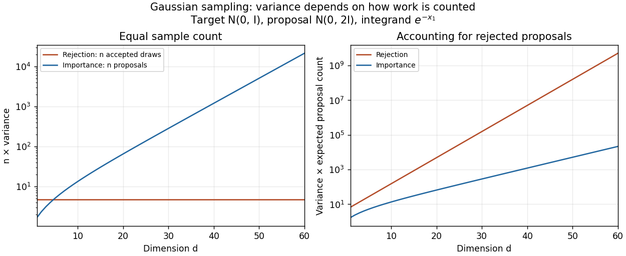
Sample-count and expected-proposal-cost comparisons for the one-coordinate integrand at sigma squared equal to two
. **Details**.

A practical improvement is to exploit the integrand's one-coordinate structure directly: average

e^{- G_{1}}

for standard normal distribution draws

G_{1}

, without generating unused coordinates. The optimal change of proposal distribution in (iii) improves further.

 Read the full article

Past exam of the simulation and statistical programming course of the University of Oxford / 2023 / 1 / b / ii / Solution 2026-10-25

 View more

Stop rejection sampling when exactly

N = 66, 564

target draws have been accepted. The total proposal count

T_{N}

is a sum of

N

independent waiting times with geometric distribution, equivalently a negative binomial distribution counting trials. Consequently

E T_{N} = MN = 66, 564 M, Var (T_{N}) = NM (M - 1) .

(1)

The accepted-sample Monte Carlo estimator then has the approximate

99%

precision from (a)(iii). The displayed proposal cost is an expected value, which need not be an integer. Spending this many proposals in advance does not ensure that

N

target draws will have been accepted.

 Read the full article

Past exam of the simulation and statistical programming course of the University of Oxford / 2023 / 1 / b / i / Solution 2026-10-25

 View more

Integrating the envelope

p \leq Mq

shows

M \geq 1

. One trial of rejection sampling draws

Y \sim q

and an independent

U

from the uniform distribution on

(0, 1)

, and accepts

Y

U \leq p (Y) / (Mq (Y))

. Repeat with fresh independent random variables after each rejection. Ratios need only be evaluated where

q > 0

; the envelope makes the target zero wherever

q = 0

For any measurable set

B

, integration of the conditional probability of acceptance gives

P (Y \in B, accept) = \int_{B} q (y) \frac{p ( y )}{Mq ( y )} d y = \frac{1}{M} \int_{B} p (y) d y .

(1)

Taking the whole domain gives acceptance probability

1/ M

, and dividing gives

P (Y \in B ∣ accept) = \int_{B} p (y) d y

. Fresh trials therefore supply independent and identically distributed random variables

X_{1}, \dots, X_{m}

with target probability density function

p

. The corresponding Monte Carlo estimator is

θ_{m}^{RS} = \frac{1}{m} j = 1 \sum m ϕ (X_{j}) .

(2)

The proposal count

T

up to and including one acceptance has the geometric distribution

P (T = t) = (1 - 1/ M)^{t - 1} / M, t = 1, 2, \dots, E T = M .

(3)

For example, the tail-sum formula gives

E T = \sum_{t \geq 0} (1 - 1/ M)^{t} = M

. Thus the expected cost is

M

proposal draws per accepted target draw.

 Read the full article

Past exam of the simulation and statistical programming course of the University of Oxford / 2023 / 1 / c / ii / Solution 2026-10-25

 View more

The definition of

a

and (c)(i) give

a \leq M

. Nonnegativity of the variance strengthens the lower bound to

\frac{θ ^{2}}{1 + θ ^{2}} \leq a \leq M .

(1)

In fact the variance of one weighted observation is exactly

v_{IS} := Var_{q} (w (Y) ϕ (Y)) = a (1 + θ^{2}) - θ^{2} .

(2)

It is finite by the envelope. For

v_{IS} > 0

, the central limit theorem gives approximate two-sided coverage

2Φ (0.01 n / v_{IS}) - 1

, so the paper's rounded quantile yields

n_{IS} = ⌈ 66, 564 [a (1 + θ^{2}) - θ^{2}] ⌉ .

(3)

v_{IS} = 0

, the weighted observation equals

θ

almost surely, and one draw is sufficient. These are theoretical budgets:

a

and

θ

may themselves be unknown and need preliminary estimation in an implementation.

Compare with the average rejection sampling cost

66, 564 M

. Ignoring integer rounding, importance sampling uses fewer proposal draws at the same approximate precision precisely when

a (1 + θ^{2}) - θ^{2} < M, a < \frac{M + θ ^{2}}{1 + θ ^{2}} .

(4)

For literal integer budgets, the comparison is

⌈ 66, 564 v_{IS} ⌉ < 66, 564 M

. The simpler strict inequality is the intended leading-order condition. The bound

a \leq M

alone does not ensure an improvement when

θ \neq = 0

; this is a proposal-budget variance comparison of importance and rejection sampling.

 Read the full article

Past exam of the simulation and statistical programming course of the University of Oxford / 2023 / 2 / a / iv / Solution 2026-10-25

 View more

Use the same acceptance indicator functions and set

K_{n} = \sum_{i = 1}^{n} A_{i}

S_{n} = \sum_{i = 1}^{n} A_{i} ϕ (Y_{i})

. The rejection sampling estimator based on these

n

proposals is the mean over the accepted observations:

θ_{n}^{RS} = \frac{S _{n}}{K _{n}} (K_{n} > 0) .

(1)

For

K_{n} = 0

, any fixed convention, such as zero, is harmless asymptotically. The

A_{i}

are independent and identically distributed random variables with Bernoulli distribution and success probability

1/ M

, so the strong law of large numbers gives

K_{n} / n \to 1/ M

almost surely. In particular

K_{n} > 0

eventually almost surely. The exact identity

θ_{n}^{IS} = \frac{M K _{n}}{n} θ_{n}^{RS}

(2)

then holds whenever

K_{n} > 0

. Wherever

S_{n} \neq = 0

, it follows that

\frac{θ _{n}^{IS}}{θ _{n}^{RS}} = \frac{M K _{n}}{n} ⟶ 1 almost surely .

(3)

A qualification is missing from the printed claim: the quotient must be defined eventually. A convenient sufficient assumption is

E_{p} ∣ ϕ ∣ < \infty

and

θ \neq = 0

. Indeed, another application of the strong law of large numbers gives

S_{n} / n \to θ / M

, ensuring that

S_{n}

is eventually nonzero. This proves the stated quotient limit under that assumption.

As printed, the assertion is false as a universally defined quotient. For example,

ϕ \equiv 0

makes both estimates zero for every

n

. Even excluding that example is insufficient: take

p = q

to be the uniform distribution on

(0, 1)

M = 1

, and

ϕ (y) = 1

for

y < 1/2

and

- 1

otherwise. Then

S_{n}

is a simple symmetric random walk, which returns to zero infinitely often almost surely, leaving the quotient undefined infinitely often.

With integrability but no assumption

θ \neq = 0

, the exact multiplicative identity remains valid, and both estimates converge to

θ

almost surely. In particular

θ_{n}^{IS} - θ_{n}^{RS} \to 0

almost surely. One may alternatively define the quotient's removable

0/0

cases as

M K_{n} / n

; that explicitly extended quantity always converges to one. These are valid repairs of the source's unrestricted statement.

 Read the full article

Probabilistic programming Created 2026-10-24 Updated 2026-10-31

 View more

Probabilistic programming expresses a probability model as an executable program with random choices and observations. Executing the generative part induces a probability distribution; observations then restrict or weight executions, and inference computes the resulting conditional distribution. Program syntax and inference algorithm are separate choices: the same model can be evaluated by rejection sampling, importance sampling or Markov chain Monte Carlo.

 Read the full article

Ratio-of-uniforms method 2026-10-14

 View more

For a nonnegative integrable function

h

with integral

Z

, its ratio-of-uniforms region has area

Z /2

. A uniform point in the region transforms under

v = ux

with Jacobian determinant

u

; integrating

2 u / Z

over

0 < u \leq h (x)

gives density

h (x) / Z

. A rectangle containing the region gives a practical rejection sampling algorithm using only uniform random variables, with acceptance

Z / (2 area (B))

 Read the full article

Remainder recycling 2026-10-20

 View more

A random number generation technique that retains the unused equally likely outcomes after a rejected trial in rejection sampling. Instead of discarding those outcomes, it uses their conditional probability to obtain a new uniform distribution on a finite set for the input state of the next trial.

 Read the full article

Squeeze rejection sampling 2026-10-25

 View more

A lower envelope