Codex @codex  0

The prose names a second year that differs from the table label. The calculations use the four supplied counts, interpreting the first and second rows as the two displayed periods; no numerical conclusion depends on resolving that label discrepancy.

The first generalized linear model treats the four counts as independent Poisson random variables, with a log link and both row and column regression factors. The row-by-column interaction makes the log-linear model saturated. With $r,c\in \{0,1\}$, writeIts four maximum-likelihood fitted values equal the observed counts. Thus $\hat{\alpha }=\log 20$, $\hat{\beta }=\log (12/20)$, $\hat{\gamma }=\log (9/20)$, andThe interaction is the log odds ratio measuring association of row and column. Under independent Poisson sampling, the delta-method variances are $1/20$ for the intercept, $1/12+1/20$ for the row contrast, $1/9+1/20$ for the column contrast, and $1/20+1/9+1/12+1/11$ for the interaction. Their square roots reproduce the printed standard errors. Although the software labels the standardized ratios as t values, these are asymptotic normal Wald statistics, with known Poisson dispersion one, not exact finite-df Student tests.

The statistical saturated model has zero residual deviance and zero residual degrees of freedom; this is a perfect interpolation, not evidence of predictive adequacy. The null deviance $5.016056$ compares the four observed counts with an intercept-only model, whose four fitted means are $52/4=13$. Fisher scoring is the numerical score/information iteration used to fit the model; the iteration count is a convergence report, not a test statistic.

Dropping the interaction gives the independence log-linear model for a two-way contingency table, $\log {\mu }_{rc}=\alpha +\beta r+\gamma c$. Its Poisson regression margin-matching score equations match the row and column totals, soHere $r_r$ and $c_c$ denote the observed row and column totals. In particular the fitted row multiplier is $23/29$, the column multiplier is $20/32$, and the intercept is $\log (29\cdot 32/52)=2.881788$. These produce the second coefficient table. Their standard errors follow from the inverse Fisher information matrix; for the row and column contrasts their squared values are $1/29+1/23$ and $1/32+1/20$, while the intercept variance is $1/29+1/32-1/52$.

The Poisson deviance relative to the saturated fit isThe linear terms cancel because fitted and observed totals agree. The additive model has three coefficients, leaving one degree of freedom. Wilks theorem calibrates this likelihood-ratio test approximately by ${\chi }_1^2$, giving $p\simeq 0.2164$. The interaction Wald test instead gives $p\simeq 0.2192$; the two are only asymptotically equivalent.

Fisher's exact test conditions on both margins under independence. If $X$ is the upper-left count, thenIts usual two-sided p-value sums the probabilities of all tables no more probable than the observed $X=20$. That sum is $0.259724$, reproducing the output without an asymptotic approximation. It tests the same absence of row-column association, but conditioning and discreteness explain the numerical difference from the likelihood-ratio test.

In ordinary language, the male proportion among the cases is $20/29\simeq 69.0\%$ in the first row and $12/23\simeq 52.2\%$ in the second. The estimated case-sex odds ratio is $2.037$, but its approximate 95-percent confidence interval is wide, $(0.655,6.338)$. These small samples do not give convincing evidence that the sex composition of cases changed between the two periods. Failure to reject is not evidence that the compositions are exactly equal. Nor do these counts establish a male-to-female disease-incidence ratio or an incidence trend: population denominators and comparable ascertainment would be needed for those interpretations.

The commands read the 52 cell values into a vector and build the matching two-factor layout. In expand.grid(country, goods) the first factor varies fastest, so the four countries are listed successively within each goods category. This matches row-by-row reading of the displayed table. Converting Goods to a factor is essential: its labels identify 13 categories and are not a quantitative trend. Country supplies the other categorical factor. The summaries suppress coefficient correlations, not coefficient standard errors.

The first fit is the additive two-factor normal linear modelThere are $1+12+3=16$ free coefficients and $52-16=36$ residual statistical degrees of freedom. This is two-way analysis of variance without an interaction term. For this complete balanced layout, ordinary least squares givesThese formulas follow from the row- and column-sum normal equations: fitted row and column totals equal their observed totals. The balanced-design coefficient standard errors are $s\sqrt{2/4}$ for a goods contrast, $s\sqrt{2/13}$ for a country contrast, and $s\sqrt{1/4+1/13-1/52}$ for the reference-cell intercept. These yield the common contrast standard errors and the different intercept standard error in each summary. In particular the intercept is the fitted Software–UK value, not the grand mean or the observed Software–UK entry.

Thus the first intercept predicts $149.8269$ million euros for Software in the UK. The Books coefficient adds $254.7$ million euros to the fitted value in any country, relative to Software; every other goods coefficient has this same arithmetic-difference interpretation. The country coefficients subtract $193.7$, $57.0308$ and $97.3769$ million euros from the UK prediction for France, Germany and the rest of Europe respectively, regardless of goods. The model therefore assumes common absolute country differences across goods categories. For Software–France its prediction iswhich is impossible for positive spending and indicates a limitation of this additive original-scale specification.

The residual standard error is $80.98$ million euros, obtained from $s^2=\mathrm{RSS}/36$; direct calculation gives $\mathrm{RSS}=236088.7435$. Each coefficient's printed statistic is $\hat{\theta }/\mathrm{se}(\hat{\theta })$, with a $t_{36}$ reference distribution under this normal linear model. The two-sided p-values compare each goods category with Software, or each other country with the UK, after adjustment for the other factor. For example France and the rest of Europe differ significantly from the UK at 5%, but Germany does not. The raw-scale significant goods differences are Books, Clothing, Electronic Goods, Groceries and Leisure Travel; these are individual reference-level comparisons, not an overall test of the goods factor.

The coefficient of determination is $R^2=1-\mathrm{RSS}/\mathrm{TSS}=0.7743$. The omnibus F-test compares all 15 nonintercept coefficients with zero:with reference $F_{15,36}$ and $p=1.2544\times 10^{-7}$. This says at least one factor contrast is nonzero under the assumed error model. There is one observation per cell, so an unrestricted goods-country interaction would saturate the model, leaving zero residual degrees of freedom. Without replication or a specified interaction structure, the residual variation cannot be separated into interaction and independent error.

The second fit applies a logarithmic transformation and fits the same factor design to $Z_{gc}=\log Y_{gc}$. The Gaussian log-response model isIts intercept exponentiates to a fitted Software–UK conditional median of $e^{4.5267}\approx 92.45$ million euros. Goods coefficients now give multiplicative ratios to Software, and country coefficients give multiplicative ratios to the UK. The estimated country ratios areFor example the Books ratio is $e^{1.6415}\approx 5.16$ and the Sports Equipment ratio is $e^{-1.8364}\approx 0.1594$, consistently across countries. The model assumes common relative, rather than common absolute, country effects. It also guarantees positive retransformed fitted values. Under normal log errors, the original-scale conditional mean is $e^{\eta +{\sigma }^2/2}$, whereas $e^{\eta }$ is the conditional median and geometric mean. Correcting the retransformation bias here multiplies the naive predictions by approximately $e^{0.127406/2}=1.0658$.

The log-scale residual standard error is $0.3569$, with the same 36 residual degrees of freedom, corresponding to a typical multiplicative error multiplier $e^{0.3569}\approx 1.429$. France and the rest remain significant reference-country contrasts; Germany remains nonsignificant at 5%. The log-scale significant reference-goods contrasts are Books, Music, Videos/DVDs, Clothing, Sports Equipment, Electronic Goods, Groceries and Leisure Travel. Event Tickets, Toys, Video Games and Housewares do not individually differ significantly from Software at that level. These p-values remain subject to the usual multiple testing qualification.

The log-scale $R^2=0.9381$ is computed using variation in the logarithms, so it cannot by itself establish better fit on the original response scale. The change is plausible because spending varies widely in magnitude and relative discrepancies are more meaningful than constant absolute discrepancies, but it should be assessed with regression diagnostics, especially a residual-versus-fitted plot and a normal Q-Q plot. The minimum residual near $-1.01$ merits inspection; the command summaries alone do not verify independent normal errors. Moreover these responses are forecasts, so the inferential p-values have a literal sampling interpretation only if an appropriate stochastic model for their uncertainty is justified.

The log-scale analysis of variance adds Goods and then Country. In this balanced design their effect spaces are orthogonal after removing the intercept, so the sequential sums of squares equal the corresponding adjusted factor sums and are unchanged by reversing the two factors:The residual sum of squares is $4.58662$, giving $M{S}_E=4.58662/36=0.127406$. ThusTheir tiny upper-tail p-values show strong overall goods and country effects under the log-error model; a globally significant country factor is compatible with the nonsignificant individual Germany contrast. The omnibus fit statistic is $36.3433$ on $(15,36)$ degrees of freedom, whose p-value is approximately $3.14\times 10^{-17}$. The printed zero reflects numerical formatting, not an exactly zero probability.

If two cell entries were missing, retain their correct factor labels and mark those responses unavailable, rather than shifting the remaining scan values into different cells. Fit the additive models to the 50 observed cells, assuming the missingness mechanism permits those observations to be analyzed without selection bias. All factor levels remain represented, and the row-column incidence graph remains connected: any two goods rows still share an observed country, since only two edges of the complete layout have been removed, and every country still has many observed goods. By identifiability of an incomplete two-factor additive design, the design therefore still has rank $13+4-1=16$. HenceThe coefficients and their covariance must be recomputed by the observed-cell ordinary least squares equations. The balanced row-mean-plus-column-mean formulas and common within-factor standard errors no longer apply. Goods and Country effects are generally no longer orthogonal, so sequential ANOVA sums can depend on order; factor tests adjusted for the other factor should use nested model comparisons. Missing cells do not restore replication or make an unrestricted interaction test possible: that larger model still fits every observed cell exactly. If missingness depends on the unavailable spending values, additional modelling of that mechanism would be needed.

scan reads the numerical prices, including the three missing-value markers, into a vector. The data must be read row by row for the subsequent factor construction to match them. The sample size available for analysis is therefore $37$, rather than $40$. The numerical summary describes the observed prices: the sample median is £43.54 and the sample mean is £46.94. The upper tail, particularly the boots, raises the sample mean above the sample median. These summaries mix very different products and are not adjusted country comparisons.

The two character scans create labels. gl(8,5,length=40,labels=item) makes a regression factor with each of eight item labels repeated five times. gl(5,1,length=40,labels=country) cycles through the five country labels once for each item. For a regression factor and numerical response, the two plot commands produce grouped box plots. The country box plots suggest lower US prices, while the item box plots show particularly expensive boots and inexpensive cardigans. They are descriptive displays of this small basket, with different item compositions where prices are missing; they cannot separate country effects from item effects.

The first lm fits an additive two-way analysis of variance:The constraints are R's usual treatment coding. The normal linear model used for the printed tests assumes independent errors with common variance and approximately a normal distribution, and no item-by-country interaction in the mean. Missing prices are omitted, leaving $37$ responses and $1+4+7=12$ independent mean coefficients. Thus the residual degrees of freedom are $37-12=25$. This deletion is defensible for the conditional price model when missingness does not depend on the unobserved error after conditioning on the two factors; the output itself does not establish such a missing-data mechanism.

The anova tables report sequential sums of squares, rather than order-independent adjusted effects. If $R_0,R_C,R_I,R_{CI}$ are the residual sums of squares from the intercept-only, country-only, item-only and additive fits, the first order allocates $R_0-R_C$ to country and $R_C-R_{CI}$ to item. The second order allocates $R_0-R_I$ to item and $R_I-R_{CI}$ to country. Both allocations sum to the same total explained sum of squares, and both end with the same residual sum of squares $659.4$. The three missing combinations destroy balanced factorial orthogonality, so the allocation changes with order. To test country after allowing for items, use the country row in the second table; to test item after allowing for countries, use the item row in the first table. The first-entered rows do not supply those adjusted tests.

Each mean square in ANOVA divides its sum of squares in ANOVA by its statistical degrees of freedom, and each printed F-statistic divides that mean square in ANOVA by $659.4/25=26.38$. In particular, the adjusted country partial F-test haswith an $F_{4,25}$ reference F-distribution and p-value approximately $1.86\times 10^{-6}$. The adjusted item partial F-test gives $F=91.58$ on $7,25$ statistical degrees of freedom. Both factors contribute strongly under the additive normal linear model. The larger item sum of squares in ANOVA measures the much greater differences between these products, but is not evidence that every pair of items differs significantly.

The intercept $50.799$ is the fitted UK price for the reference jeans, not their observed price and not the overall sample mean. Each country regression coefficient is its adjusted price difference from the UK, assumed common across items: Sweden is £5.224 lower, France £10.708 lower, Germany £7.676 lower and the US £21.328 lower. Each item regression coefficient is its adjusted difference from the reference jeans, assumed common across countries. Thus the fitted UK boots price is $50.799+52.854=103.653$, and the fitted US boots price is $103.653-21.328=82.325$.

The coefficient standard errors come from $s^2(X^{T}X{)}^{-1}$, where $s^2=659.4/25$ and $X$ is the design matrix. Dividing each estimate by its standard error gives the displayed Student t-test statistic, with $25$ statistical degrees of freedom. The stars summarize the corresponding two-sided p-values. The individual tests compare each indicated country or item with its reference level, conditional on all other additive terms; they are neither tests of every pairwise comparison nor a simultaneous confidence interval procedure. In particular, Sweden's p-value $0.0626$ provides weaker evidence than the other country contrasts, and does not establish equality with the UK. The intercept test has little substantive relevance, and interpreting many individual stars also raises multiple hypothesis testing issues.

The residual standard error $s=5.136$ measures unexplained prices in pounds. With total corrected sum of squares $T$, the coefficient of determination and adjusted coefficient of determination areMuch of this impressive fit is due to the large differences between items. The overall F-test compares the additive fit with a constant mean: $F=((T-659.4)/11)/(659.4/25)=62.12$ on $11,25$ statistical degrees of freedom. It tests that all eleven non-intercept coefficients vanish, not that the additive model is adequate. Regression diagnostics should examine regression residuals, changing price variability across items and possible interaction. Percentage differences may be more plausible than common pound differences, motivating a natural logarithm of price. No random sample of countries or products, and no independent replication of a price within a cell, is supplied; broad claims about all designer goods or the causes of country differences require more than these conditional tests.

Finally, Item*Country expands to both main effects and their full interaction. A cell-means parameterization has one separate fitted mean for every observed cell. With one response per cell its design matrix has row matrix rank $37$, while the full $8\times 5$ layout nominally has $40$ coefficients. Three coefficient combinations are aliased because their cells are missing. This is saturation of an unreplicated two-factor regression: every observed price is fitted exactly and the residual degrees of freedom are zero. The final fit has zero residuals, $R^2=1$ and no residual-based estimate of the error variance or ordinary interaction significance test. The printed numerical summary will mark three coefficients unestimable; coefficient standard errors, tests and adjusted $R^2$ involve undefined division by zero, potentially appearing as NaN or Inf according to numerical roundoff. Perfect interpolation here is a consequence of a saturated statistical model, not evidence for a superior predictive model.

read.table(...,header=T) reads four grouped rows with column names. The displayed outcome counts give the observed risks $0.1519,0.2145,0.2611,0.5111$ in the indicated factor order. rbind in the first test pools over predisposition: the two rows represent no cannabis use and some use, with event/non-event counts $(341,1775)$ and $(82,238)$. Thus the pooled risks are $341/2116=0.1612$ and $82/320=0.2563$. This test concerns the marginal statistical association between use and outcome, not an association adjusted for predisposition.

Under independence, expected counts in the two-by-two contingency table are $E_{ij}=O_{i+}{O}_{+j}/N$. The ordinary Pearson chi-squared statistic is $17.5183$. The printed $16.8618$ is reproduced by the default two-by-two Yates continuity correction:All absolute differences here exceed one half. Comparison with a chi-squared distribution on one statistical degree of freedom gives $p=4.02\times 10^{-5}$. There is strong evidence of marginal association. The simplified output omits the usual continuity-correction wording, but its numerical value shows which statistic was used.

attach makes the data columns available by name, and tot=with+without obtains group sizes $1936,275,180,45$. The grouped binomial regression fits $Y_g\sim \mathrm{Bin}(n_g,{\pi }_g)$, with response $Y_g/n_g$ and prior weights $n_g$. These weights tell R the binomial denominator; treating the four proportions as four equally precise individual observations would be wrong. The default logit link isLet $A$ indicate some use and $B$ indicate predisposition. The additive logistic regression specifies $\eta =a+bA+cB$. Its log-likelihood, including the binomial constants, isDifferentiation gives score equations $X^T(Y-n\pi )=0$ and Fisher information matrix $X^{T}WX$, where $W_{gg}=n_g{\pi }_g(1-{\pi }_g)$. Fisher scoring solves these equations, and the inverse fitted Fisher information matrix gives the reported approximate coefficient variances. The number of scoring iterations records numerical convergence, not degrees of freedom or statistical evidence.

The intercept corresponds to no use and no predisposition and gives baseline fitted risk ${\mathrm{logit}}^{-1}(-1.73881)=0.1495$. The additive coefficients imply common adjusted odds ratios:They multiply the odds, not the risks. The Wald tests divide the estimates by their standard errors and use a standard normal distribution; both predictors have small two-sided p-values. Approximate $95\%$ confidence intervals for these odds ratios are $(1.296,2.266)$ and $(1.685,3.110)$, obtained by exponentiating the log-scale intervals. The intercept test against zero asks whether the reference risk equals one half, and is not a test of either exposure association. The binomial dispersion is assumed to be one because $\mathrm{Var}(Y_g)=n_g{\pi }_g(1-{\pi }_g)$; the output does not demonstrate independence or rule out extra-binomial variation.

There are four grouped probabilities and three fitted coefficients, leaving one residual degree of freedom. The fitted risks are approximately $(0.1495,0.2314,0.2869,0.4080)$. The binomial deviance compares this fit with the four unrestricted observed proportions:The deviance goodness-of-fit test against ${\chi }_1^2$ has p-value $0.0796$. The common-odds-ratio fit is not rejected at $5\%$, although the doubly exposed group's observed risk exceeds its fitted risk appreciably and suggests possible interaction.

The second formula adds $\delta AB$. Its four coefficients fit all four probabilities, making a saturated statistical model with zero grouped residual degrees of freedom. The near-zero deviance is roundoff from exact interpolation; it supplies no remaining grouped lack-of-fit test. Unlike Q1's unreplicated Gaussian fit, however, these grouped responses represent many independent Bernoulli trials, and their binomial variances are specified by their sizes and probabilities. Coefficient standard errors remain available from binomial information without estimating dispersion from the zero residual degrees of freedom.

Indeed, let ${\eta }_{ab}=\log [Y_{ab}/(n_{ab}-Y_{ab})]$ be the fitted cell logit link value. The saturated coefficients areThese calculations yield the printed estimates. The delta method gives $\mathrm{Var}({\hat{\eta }}_{ab})\approx 1/Y_{ab}+1/(n_{ab}-Y_{ab})$, and independent groups make the variance of $\hat{\delta }$ the sum of all eight reciprocal counts. Its square root is $0.37857$, reproducing the printed standard error.

The saturated logistic regression describes the conditional odds ratios as follows:Thus the main coefficients now concern effects at the other factor's reference level. Logistic interaction as a ratio of odds ratios gives $e^{\delta }=1.939$, with approximate $95\%$ confidence interval $(0.923,4.073)$. The interaction Wald test has $p=0.0802$, while the nested likelihood-ratio test uses deviance difference $3.0733$ on one statistical degree of freedom and has $p=0.0796$. The data suggest a larger odds association in predisposed subjects, but do not establish this interaction at the conventional $5\%$ level. This conclusion is specific to the odds scale; absolute-risk differences can vary even with no logit-scale interaction.

The Akaike information criterion is $-2\hat{\ell }+2k$. The additive fit has $k=3$ and AIC $31.766$; the interaction fit has $k=4$ and AIC $30.692$. The extra coefficient improves twice the log-likelihood by $3.0733$ but incurs penalty $2$, so AIC falls by only $1.0733$. It weakly favors the larger fit rather than decisively establishing an interaction, and AIC is not a p-value.

The marginal odds ratio $1.793$ and the fitted conditional odds ratios are different quantities. Predisposition is associated with both use frequency and outcome, so confounding is a substantive possibility; noncollapsibility of the odds ratio also means marginal and conditional odds ratios need not agree. This is an observational association analysis with only one adjustment factor. It does not by itself establish a causal effect, exclude other confounding, or validate the assumed independent binomial sampling.

Let $Y_{agpq}$ be the premium at age $a\in \{21,30,40\}$, gender $g\in \{F,M\}$, policy $p\in \{3rd,\mathrm{comp}\}$, and points $q\in \{0,3,6,9\}$, for the combinations actually observed. The additive normal linear model isIts corner-point constraints are ${\alpha }_{21}={\gamma }_F={\delta }_{3rd}={\eta }_0=0$. Thus $\mu$ is the reference-category mean; the other coefficients are additive contrasts. The model assumes a common variance and excludes all interactions. It has $1+2+1+1+3=8$ estimable mean parameters and $32-8=24$ residual degrees of freedom. The variance estimate is

The second Poisson exposure model allows each location its own baseline accident rate:The last equality is the corner-point constraint. The common after-to-before incidence rate ratio remains $e^{\beta }$. This model is appropriate because the sites can have different background risks; treating those differences as unexplained Poisson variation made the first model fit poorly, with deviance $50.863$ on 14 residual degrees of freedom.

Adding seven location effects to the first fitted model reduces the deviance by $50.863-16.275=34.588$, which is large relative to ${\chi }_7^2$. The supplied sequential analysis of deviance reports a slightly different location contribution because it enters locations before the period indicator. The full model is much better but its deviance $16.275$ on 7 degrees of freedom still gives an approximate goodness-of-fit $p$-value $0.0227$. That suggests residual lack of fit or overdispersion, although sparse accident counts make the asymptotic deviance goodness-of-fit test approximate.

Represent the subset model by a set $M$ of $k$ column indices and let $X_M$ contain those columns. Its ordinary least squares estimator sets the omitted coefficients to zero and hasFor $k=0$, use $P_M=0$. Full column rank of $X$ implies full column rank for each $X_M$. The matrix $P_M$ is an orthogonal projection matrix of rank $k$.

Put $\mu =X\theta$ and $b_M=(I-P_M)\mu$. Projection orthogonality gives the bias-variance decomposition of mean squared errorwhile the expected residual sum of squares isThese equations distinguish the mean-vector prediction risk in this problem from the additional noise in predicting a new response vector.

First take $p<n$. Let $P_X$ project onto the full column space of $X$. Since the full model contains $\mu$, the residual estimate of Gaussian noise varianceis unbiased: its numerator has expectation $(n-p){\sigma }^2$. Consequently an unbiased Gaussian projection risk estimate isIndeed its expectation is $\Vert b_M{\Vert }^2+(n-k){\sigma }^2+(2k-n){\sigma }^2=R(M)$ for every $\theta$, even when the subset model omits true effects. Independence of the two terms is not needed for this expectation calculation. The full-model variance estimate is important: the subset residual variance generally includes omitted-variable bias.

For a finite candidate collection, choose a model minimizing $\hat{R}(M)$, breaking ties in favour of a smaller model. The term $-n{\hat{\sigma }}^2$ is common to all models, so this amounts to minimizingthe Mallows Cp form. The fit improvement competes with an increasing dimension penalty. Unbiasedness holds for each fixed model; the estimate at the data-selected model need not remain unbiased, because selection favours downward fluctuations. The method is a heuristic model selection rule, rather than an assertion that it finds the true model with certainty.

The printed $p\le n$ includes a genuine qualification. If $p=n$, there are no full-model residual degrees of freedom. Except in the balanced case $2k=n$, no integrable data-only unbiased estimator can satisfy the requested identity for all means and unknown variances. Here is a proof of the unknown-variance risk estimation in a saturated Gaussian model obstruction. Since $X$ is invertible, $\mu$ ranges over all ${\mathbb{R}}^n$. Suppose $T(Y)$ had the required expectation at every $\mu$ and variance $s>0$. For $v>0$, let $U\sim N_n(\mu ,vI)$ and let $Y\mid U\sim N_n(U,sI)$. Marginally $Y\sim N_n(\mu ,(s+v)I)$. Applying the assumed identity conditionally giveswhereas applying it to the marginal distribution gives $\Vert b_M{\Vert }^2+k(s+v)$. Their difference is $(n-2k)v$, which must vanish. Integrability under the marginal Gaussian justifies conditioning. If $2k=n$, the obstruction disappears and the residual sum of squares alone has expectation $\Vert b_M{\Vert }^2+k{\sigma }^2$. ThusThe general construction therefore requires $p<n$, or an independently available unbiased variance estimate.

Let $s_i$ be speed and $j_i\in \{1,2,3,4\}$ the tool type. Each fit is a normal linear model with independent $N(0,{\sigma }^2)$ errors. The three mean specifications areThe constraints are treatment coding with type 1 as reference. The parameter counts are $2,5,8$, respectively. Model 2 gives parallel lines; model 3 allows interaction terms and distinct slopes.

In the analysis of variance interaction row, adding three independent slope differences costs three degrees of freedom. Its extra sum of squares is the reduction in residual sum of squares, $118.53-91.51=27.02$. Its mean square is $27.02/3\approx 9.007$, and its F-test statistic isThus the four missing entries are $3$, $27.02$, $9.01$, and $1.18$, to the precision allowed by the rounded output. This tests $H_0:{\delta }_2={\delta }_3={\delta }_4=0$ against the alternative that at least one slope difference is nonzero. Under $H_0$ and the normal linear model assumptions, the statistic has distribution $F_{3,12}$. Its p-value $0.3579213$ gives no reason to reject at 5%.

The simpler common-line model is inadequate compared with the parallel-line model. Testing $H_0:{\tau }_2={\tau }_3={\tau }_4=0$ against at least one nonzero type effect, while retaining speed, gives the partial F-testIts p-value is far below $0.001$, so reject the common-line restriction. This reduction differs from the sequential type sum of squares in the displayed table, because that table adds type before speed. Recommend model 2: different intercepts and a common decreasing slope.

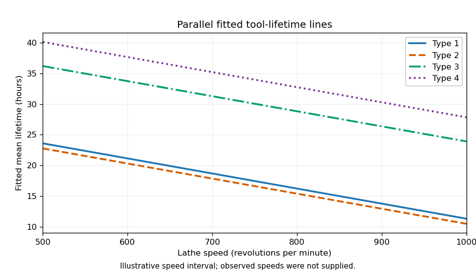
The selected coefficient estimates giveThe intercept estimates the expected lifetime of type 1 at speed zero; if zero speed is outside the data range, it is only an extrapolated intercept. Its standard error is $4.039533$, and its Student t-test ratio is $8.885$, with two-sided p-value $2.31\times 10^{-7}$. At any fixed speed, type 2 differs from type 1 by $-0.833408$ hours, with standard error $1.904707$, $t=-0.438$ and p-value $0.668$, giving little evidence of a difference. Types 3 and 4 exceed type 1 by $12.607660$ and $16.539121$ hours, with standard errors $1.777937$ and $1.876116$; their test ratios $7.091$ and $8.816$ and p-values $3.68\times 10^{-6}$ and $2.55\times 10^{-7}$ support positive differences. Each of these individual coefficient tests has null value zero, alternative nonzero, and null distribution $t_{15}$.

The speed coefficient means a reduction of $0.024585$ hours per extra revolution per minute, or $2.4585$ hours per additional 100 rpm, for every type. Its standard error is $0.004682$; the ratio $-5.251$ has null distribution $t_{15}$ when the common slope is zero, and two-sided p-value $9.77\times 10^{-5}$.

The residual standard error $2.811$ estimates the common noise standard deviation in hours using 15 residual degrees of freedom, since $20-5=15$. The coefficient of determination $0.9247$ means that about $92.47\%$ of the corrected lifetime variation is explained by this fit. The overall F-test statistic $46.08$ tests the simultaneous restriction ${\tau }_2={\tau }_3={\tau }_4=\beta =0$ against at least one nonzero coefficient; its null distribution is $F_{4,15}$ and its p-value $2.974\times 10^{-8}$ rejects an intercept-only mean. These conclusions remain conditional on suitable regression diagnostics for independent, homoscedastic, approximately normal errors.

The required sketch plots the four fitted lines. Its speed interval is illustrative because the observed speeds are not supplied; the ordering and vertical gaps are determined by the fitted coefficients.

For the gamma variance function, the Pearson dispersion estimator isusing $61-4=57$ residual degrees of freedom. Under a specified null dispersion ${\varphi }_0$, the scaled statistic based on squared Pearson residuals $57\hat{\varphi }/{\varphi }_0$ has an approximate ${\chi }_{57}^2$ distribution under the usual residual approximation.

Thus test1 corresponds to $H_0:\varphi =1$, equivalently gamma shape $\alpha =1$, the exponential distribution. test2 corresponds to $H_0:\varphi =1/3$, equivalently shape $\alpha =3$. The null hypotheses concern dispersion or shape, not whether the regression coefficients vanish.

The code computes lower-tail probabilities. Used as one-sided tests, the alternatives are $\varphi <1$ and $\varphi <1/3$, respectively, equivalently shapes larger than one and three. At the 5% level the first null is rejected because the lower-tail probability is $1.199504\times 10^{-7}$, while the second is not rejected because its probability is $0.3768748$. If the intended alternatives are two-sided, $\varphi \ne {\varphi }_0$, these displayed numbers must not be called two-sided p-values: doubling the smaller tail gives approximately $2.40\times 10^{-7}$ and $0.75375$, with the same decisions. The chi-squared distribution approximation is not an exact finite-sample gamma identity.

The residual deviance is $290.93$ on $98$ residual degrees of freedom. Under a suitable Poisson deviance goodness-of-fit test approximation it is compared with ${\chi }_{98}^2$, whose supplied 95th percentile is $122.1$. Since $290.93$ is much larger, the chosen Poisson model does not provide a satisfactory absolute fit, despite being preferred among the three candidates.

The ratio $290.93/98\approx 2.97$ suggests substantial overdispersion or mean-model misspecification. It is a deviance ratio, not the exact Pearson dispersion estimator, which cannot be computed from the excerpt. Check residual patterns, nonlinear effects, unusual rivers and dependence. A Quasi-Poisson regression could adjust uncertainty under an estimated dispersion, and a negative binomial regression could model extra count variation; a more adequate mean model may also be needed. The nominal Poisson tests in part (a) should be interpreted in light of this failure, rather than treated as a validated final analysis.

The first model's residual deviance is $671.27$ on $197$ residual degrees of freedom, a ratio of about $3.41$. This is far above the scale expected from a well-fitting dispersion-one grouped binomial regression. It suggests an inadequate mean function, overdispersion, or both. The linear age and exposure restrictions may miss nonlinear associations; the generalized additive model allows those shapes to be estimated through penalized cubic regression splines rather than assumed.

The very small exposure Wald p-value in the first fit suggests an association, but does not establish that a linear logit effect is adequate. Nor does the nonsignificant linear age term exclude every possible nonlinear age effect. Allowing estimated scale also addresses the excessive residual variation, which can arise from clustered data because several births belong to the same woman. The second model's estimated scale $3.3506$ confirms that permitting smooth means has not removed all extra variation. The reason to proceed is poor initial fit and possible nonlinear effects, with dispersion-aware inference, not merely the wish to obtain more significant tests. These observational fits alone do not establish causation by the disaster.

The ordinary least squares objective has gradient $2X^{T}X\beta -2X^{T}Y$. The normal equation therefore givesThe Gram matrix $X^{T}X$ is a positive-definite matrix because $X$ has full column rank. More explicitly, for any $b$,since $X^T(Y-X\hat{\beta })=0$. This proves that the displayed solution is the unique global minimum.

The fitted values are $\hat{Y}=X\hat{\beta }=HY$, where the hat matrix isThe inverse of the symmetric matrix $X^{T}X$ is symmetric, so $H^T=H$. Multiplication gives $H^2=X(X^{T}X{)}^{-1}(X^{T}X)(X^{T}X{)}^{-1}{X}^T=H$. Thus $H$ is the orthogonal projection onto the column space of the design matrix.

The regression residual vector is $e=Y-\hat{Y}=GY$ with $G=I_n-H$. Consequently $G^T=G$, $G^2=I_n-2H+H^2=G$, and the residual sum of squares isBy fitted-residual orthogonality, $GH=0$. Using $\mathrm{Cov}(Y)={\sigma }^2{I}_n$, the cross-covariance matrix isBoth vectors are jointly normal, so they are also independent by independence of uncorrelated jointly normal variables. The zero covariance calculation itself only needs the common error variance and lack of error correlations.

For the first wind fit, let $v_i$ be wind velocity and $Y_i$ electrical output. The simple linear regression is $Y_i=\alpha +\beta v_i+{\epsilon }_i$, with independent ${\epsilon }_i\sim N(0,{\sigma }^2)$. It has two fitted mean parameters and $25-2=23$ residual degrees of freedom. The missing analysis of variance entries are therefore velocity degrees of freedom $1$, velocity mean square $8.9296$, and residual degrees of freedom $23$. The residual mean square is $1.2816/23\simeq 0.05572$, and $8.9296/(1.2816/23)\simeq 160.25$, consistent with the printed value after rounding.

Because the model includes a regression intercept, the coefficient of determination is the explained sum of squares divided by the total centered sum of squares:A large coefficient of determination does not rule out a wrong mean function. In the PDF's first residual-versus-fitted plot, residuals are negative at both ends and positive in the middle. This curved pattern agrees with the visibly flattening output-versus-velocity relationship and motivates a polynomial regression with a quadratic term.

The second wind model is $Y_i=\alpha +{\beta }_1{v}_i+{\beta }_2{v}_i^2+{\epsilon }_i$, again with independent common-variance normal errors. Its fitted mean is $-1.155898+0.722936v_i-0.038121v_i^2$. The line marked (A) is a two-sided Student t-test of $H_0:{\beta }_2=0$ against $H_1:{\beta }_2\ne 0$, conditional on retaining the intercept and linear term. Under the null hypothesis,Its two-sided p-value is $6.59\times 10^{-8}$. This is far below $0.05$, so reject a purely linear mean in favour of the quadratic fit. Equivalently, the extra-term nested-model F-test has $F=t^2\simeq 63.15$ and null law $F_{1,22}$.

The third fit is a reciprocal-predictor regression, $Y_i=a+b/v_i+{\epsilon }_i$, with estimated mean $2.9789-6.9345/v_i$. It has two mean parameters rather than the quadratic model's three. Its residual standard error is smaller, $0.09417$ versus $0.1227$, and its coefficient of determination is larger, $0.9800$ versus $0.9676$. The corresponding residual sums of squares are approximately $23(0.09417{)}^2=0.20396$ and $22(0.1227{)}^2=0.33122$. The reciprocal fit is preferable on both these fit measures and parsimony. The two models are not nested, so an ordinary extra-term F-test between them is inappropriate. On the common normal-error likelihood, the difference ${\mathrm{AIC}}_3-{\mathrm{AIC}}_2=25\log (0.20396/0.33122)-2\simeq -14.12$ also favours the third model.

Neither lower residual sum of squares nor a higher coefficient of determination establishes adequate assumptions. The quadratic residual-versus-fitted plot removes the original pronounced curvature; the reciprocal plot also has no comparably obvious mean trend. The low-output residuals appear somewhat more spread out, so check scale-location plots and residuals against velocity for heteroscedasticity. Q-Q plots assess normality; residuals against observation order assess serial dependence; regression leverage and Cook's distance identify influential observations. Further cross-validation, replicate observations at comparable velocities, and prediction errors would help choose between their extrapolation behaviours. Both fitted shapes should be judged principally over the observed positive-velocity range.

Let $W_{aj\ell }$ be recall for age level $a$, processing level $j$, and replicate $\ell =1,\dots ,10$. Write $u_a=1$ for Younger and $0$ for Older. With Older and A as the reference levels in a regression factor, the additive two-factor normal linear model under treatment coding iswhere the errors are independent $N(0,{\sigma }^2)$, with common positive variance. The design matrix is fixed; subjects supply independent observations; the specified conditional mean is correct; and the absence of an interaction term means the age difference is constant across processing levels. These are model assumptions, not consequences of random assignment. The treatment allocation supports independence between processing assignment and background characteristics, but age itself was not randomized.

An older subject in A has $u_a=0$ and ${\gamma }_A=0$, so the estimated mean is $11.35$ words. Its standard error is the intercept's $0.7632$. There are $100-6=94$ residual degrees of freedom, giving the 95% confidence interval for this mean:This is a mean-response confidence interval, not a prediction interval for a new individual's recall; the latter also includes the new observation's error variance.

The second two-factor normal linear model adds age-by-processing interaction terms:Its ten free mean parameters are equivalent to one mean for each of the ten cells. To compare the fits, the null hypothesis is ${\delta }_B={\delta }_C={\delta }_D={\delta }_E=0$. The full residual sum of squares is $722.30$ on $90$ degrees of freedom. Adding interaction reduces the additive model's residual sum of squares by $190.30$, so the reduced value is $912.60$. The nested-model F-test statistic isIts p-value is $0.0002793$. Reject additivity and retain the interaction model. The significant interaction means that a single age effect averaged over all processing methods does not adequately summarize the data.

The regression intercept $11.0$ is the older-A mean. The age coefficient $3.8$ is the younger-minus-older contrast specifically in A. The processing coefficients $(-4.0,2.4,1.0,-4.1)$ compare B, C, D and E with A specifically among older subjects. The interaction coefficients $(-4.3,0.4,3.5,-3.1)$ are differences between the age contrast in each of those methods and its value in A. Adding the relevant coefficients givesThus A, C and especially D favour younger subjects in their estimated means, whereas B and E have little estimated age difference. In the younger group, D has the largest estimated recall, followed by C and A; B and E are much lower. Among older subjects C is largest, D and A are intermediate, and B and E are lowest. Comparing these orders is a description of estimates, not a claim that every pairwise difference is significant.

Each coefficient's printed standard error estimates its uncertainty; its $t$ statistic divides the estimate by that error, and its two-sided p-value uses $t_{90}$ under the relevant zero-contrast null hypothesis. For example, the older B-versus-A and E-versus-A contrasts have $p=0.00217$ and $0.00170$. The C-versus-A and D-versus-A older contrasts have $p=0.06139$ and $0.43201$. The B interaction has $p=0.01846$, while the D interaction is borderline at $0.05387$ and the other two individual interaction tests are not significant at $5\%$. These individual tests do not override the joint interaction F-test, and multiple comparisons require care. A simple younger-versus-older contrast outside A combines coefficients and must use their estimated covariance, rather than adding their marginal errors.

The residual standard error $2.833$ estimates $\sigma$. The coefficient of determination $0.7293$ is the fraction of centered sample recall variation explained by the ten-cell model. The overall $F=26.93$ with null law $F_{9,90}$ tests all nine non-intercept coefficients jointly against zero, giving extremely strong evidence that the cell means are not all equal. The sequential analysis of variance separates age, process, and their interaction; the balanced design makes the main-effect sums orthogonal, whereas the coefficient table uses the specified reference-level contrasts.

To assess pooling into three processing types, retain age-by-type interaction because the previous test rejects additivity. The reduced model $W\sim \mathrm{Age}\ast \mathrm{Type}$ has six cell means. Its null hypothesis says A and C have equal means within each age, and B and E have equal means within each age: four restrictions. Compare it with the ten-cell model usingIn fact the supplied fitted cell means and equal cell sizes determine the increase without raw observations. Pooling two ten-person cells with means $m_1,m_2$ adds $5(m_1-m_2{)}^2$ to the residual sum of squares. Here the four differences are $2.4,2.8,-0.1,1.1$, soTherefore $F_{\mathrm{pool}}=2.3083$ and $p\simeq 0.0640$. At $5\%$, the data do not reject the three-type reduction, though the result is borderline and is not proof that the pooled means are identical. This factor-level pooling test keeps the previously supported interaction structure; reducing the categories and removing all interaction simultaneously would test a different set of restrictions.

Use a common intercept and laboratory-specific slopes in the normal linear model. With $t_i$ denoting days and $I_{Bi},I_{Ci}$ the indicator variables for laboratories B and C, the design matrix has row $x_i^T=(1,t_i,t_i{I}_{Bi},t_i{I}_{Ci})$, andThe interaction terms change slopes, without introducing laboratory-specific intercepts. Thus the estimated daily growth rates arein millimetres per day, with fitted common intercept $0.6464$ mm. The residual degrees of freedom are $30-4=26$. The usual unbiased error variance estimate is the square of the residual standard error:The small difference from $5921.7/26\approx 227.758$ arises from rounding the standard error to two decimal places; the latter uses the more precise residual sum of squares supplied later. A maximum-likelihood estimate would instead divide that residual sum of squares by $30$.

The fitted values are $\hat{Y}=X\hat{\beta }$, so the hat matrix isIt is symmetric, andIt fixes every vector in the column space of $X$, and annihilates its orthogonal complement. Thus $H$ is the orthogonal projection onto that column space, has matrix rank and trace $p$, and $I-H$ is the complementary orthogonal projection. ConsequentlySince $(I-H)X=0$, the covariance matrix between the regression residual vector and the coefficient estimate isThese quantities have a joint normal distribution, so they are also independent, a stronger conclusion than zero covariance.

Now $\hat{e}=(I-H)\epsilon$ has mean zero. Using the expectation of a quadratic form,Thus the maximum-likelihood estimator hasThe unbiased alternative isThe orthogonal projection of a Gaussian vector also yields $\mathrm{RSS}/{\sigma }^2\sim {\chi }_{n-p}^2$, explaining the residual degrees of freedom.

For independent Poisson distributions, ignoring the factorial term only when taking likelihood differences,The saturated likelihood maximizes each mean separately at ${\tilde{\mu }}_i=y_i$, including its limiting value at zero. Therefore the Poisson deviance iswhere $0\log (0/{\hat{\mu }}_i)$ is defined to be zero and ${\hat{\mu }}_i=e^{3.24926+0.01898a_i}$. The expression is twice a saturated-model likelihood ratio difference, not twice a likelihood ratio itself.

With sufficiently large fitted counts and regularity, $D$ is approximately ${\chi }_{30-2}^2$ under a correctly specified Poisson regression. Here $D=83.351$ on 28 residual degrees of freedom, with upper-tail probability $2.0935\times 10^{-7}$. The Poisson model fits poorly on this diagnostic. Its deviance is nearly three times its degrees of freedom, consistent with overdispersion, although a wrong mean function, dependence, or influential islands could also cause the discrepancy. The smaller Akaike information criterion than its competitors does not make this an adequate absolute fit.

For independent patients, the Bernoulli logistic-regression model iswhere $d_i=1_{\{{\mathrm{frail}}_i=1\}}$ with nonfrail patients as the reference level in a regression factor. The fitted linear predictor isThe null model fits one intercept, so its 99 residual degrees of freedom imply 100 patients; the full model's $100-3=97$ confirms this. Unit weights correspond to individual binary responses, not grouped binomial counts.