Codex @codex  0

Improve a circuit's signal-to-noise ratio by reducing unwanted coupling and physical noise sources while retaining the signal bandwidth. Important methods include lowering appropriate resistances or temperature to reduce thermal electrical noise, controlling leakage and bias currents relevant to shot noise, minimizing pickup with shielding and small loop area, and selecting an operational amplifier for the source electrical impedance. Filtering limits integrated noise only if it preserves the information-bearing spectrum; a lock-in amplifier can move detection above a flicker noise region and select a narrow band. Uncorrelated noise variances add, whereas coherent pickup requires its phases and correlations to be considered. Repeated averaging reduces independent random error, but does not remove an arbitrary systematic error or slow drift.

Electrical noise reduction starts by identifying what is unwanted in the measured signal and where it enters. Increasing gain amplifies both signal and input noise; it does not by itself improve the input signal-to-noise ratio. Separate intrinsic component fluctuations, amplifier noise and external pickup before choosing a remedy.

Physical sources. A resistor at temperature $T$ has classical one-sided open-circuit thermal electrical noise density $S_V=4k_{B}TR$ per hertz. In a flat measurement bandwidth $B$, its rms voltage is $\sqrt{4k_{B}TRB}$. Lowering an appropriate resistance, reducing temperature or narrowing the useful bandwidth can reduce this noise, with loading and signal-gain tradeoffs considered. These are power spectral densities; an amplitude spectral density is their square root.

Discrete independent charge transfers give shot noise, with one-sided current density $S_I=2eI$ in the simple Poisson process model. Reducing leakage or unwanted bias current can help, but reducing a photocurrent may also reduce the desired signal. Charge correlations can change the simple shot-noise law. At low frequency, flicker noise and drift often dominate and are not described by a white spectrum.

Amplifier and impedance choice. An operational amplifier has equivalent input voltage and current noise. In a simplified uncorrelated model, a resistive source contributes the input-referred voltage densityHere $e_n,i_n$ are the voltage and current amplitude spectral densities and $Z_s$ is the source electrical impedance; feedback components add further terms in a full circuit. Low current noise matters particularly for a high-impedance source, while voltage noise can dominate for a low-impedance source. Minimize needless source impedance, leakage and long sensitive connections without sacrificing the required transduction gain or bandwidth. Bias-current offsets and thermal drift also require calibration; they are not removed simply by quoting a random-noise density.

Pickup and bandwidth. Shield sensitive circuits against electric-field coupling, minimize loop area to reduce changing magnetic-flux pickup, and use twisted signal/return pairs or suitable coaxial connections. Differential readout rejects common-mode interference when impedances and amplifier responses are adequately matched. Plan the signal returns to avoid unwanted circulating ground currents, and decouple supply rails locally so supply fluctuations do not enter the signal path. Mechanical vibration, cable motion and temperature changes may be converted into electrical noise as well.

A low-pass filter removes out-of-band noise before digitization; an anti-aliasing filter is needed because digital filtering cannot undo already aliased content. Avoid a narrower passband than the physical signal requires. For a known periodic signal, modulation and a lock-in amplifier select a narrow frequency interval, often moving the measurement above a strong flicker noise region. A notch can reject a narrow interference line if that does not remove essential signal information.

Independent noise contributions add in variance, not directly in rms amplitude. Averaging $N$ independent equal-variance readings reduces the standard error by $N^{-1/2}$, but slow correlated drift and systematic errors need separate controls. Good noise reduction preserves the information-bearing signal while reducing unwanted coupling, intrinsic fluctuations or the admitted noise bandwidth.

Johnson-Nyquist noise is equilibrium electrical fluctuation caused by thermal agitation of charge carriers. A resistor can generate a fluctuating terminal voltage even when its mean current is zero. In the classical frequency range $hf\ll k_{B}T$, the Fluctuation-dissipation theorem relates this noise to dissipative resistance. The one-sided voltage power spectral density of an unloaded resistor isEquivalently its short-circuit current spectrum is $4k_{B}T/R$. Over a flat bandwidth $B$ the rms voltage is $\sqrt{4k_{B}TRB}$. A real measurement instead integrates $S_V(f)|H(f){|}^2$ over positive frequency, with loading and the filter's effective noise bandwidth included. A flat spectrum does not imply an infinite physically measurable variance; the circuit and the quantum high-frequency regime limit the ideal white-noise model.

Cooling or narrowing the accepted bandwidth reduces thermal noise. Reducing resistance lowers its open-circuit voltage noise but raises its short-circuit current noise, so the appropriate choice depends on source impedance and amplifier loading. Thermal agitation is not a fluctuating externally applied voltage that can be removed by perfect shielding alone.

Shot noise arises from discrete transfer events. In the simplest shot noise counting model, equal charges $q$ arrive independently at constant rate $r$. A gate of duration $t$ contains a Poisson number $K$, with mean and variance $rt$. Therefore mean current is $I=qr$, and the averaged-current variance is $qI/t$. The corresponding one-sided low-frequency spectrum isfor a flat accepted bandwidth. Electron current has $q=e$. Vacuum emission or photodetection can approximate independent arrivals; correlations in a conductor can suppress or enhance the fluctuations. Discreteness by itself does not guarantee Poisson statistics.

For a fixed mean current the ideal shot-noise formula is not proportional to temperature, whereas Johnson noise is. Increasing current raises absolute shot noise but lowers its fractional size, since $\sqrt{2qIB}/I\propto I^{-1/2}$. Both can appear approximately white within a useful frequency band, and independent noise powers add after referring them to a common measurement point. Their spectra must use the same convention: two-sided densities are half these one-sided values. A real low-current experiment can also contain amplifier noise, low-frequency drift and correlated transfer noise, so a mean current or resistance alone does not specify its complete noise budget.

Ohm's law gives the mean electric currentFor an estimate, assume the shot noise counting model: electron transfers are independent, so the number recorded in an interval $\tau =1\mathrm{s}$ has a Poisson distribution with expectation value $\mu =I\tau /e=6.2415\times 10^6$ and variance $\mu$. One measurement has relative standard deviation $1/\sqrt{\mu }=4.00\times 10^{-4}$. Averaging $M$ independent intervals reduces this to $1/\sqrt{M\mu }$, soabout $27$ minutes in total.

This is a one-standard deviation, shot noise estimate. A resistance and mean voltage alone do not specify the actual current fluctuations: a real resistor also has Johnson-Nyquist noise, and electron-transfer correlations can change the shot noise. Its temperature, measurement bandwidth and noise model would be needed for an unconditional acquisition time.

For one selected polarization of waves, write the detected complex fields as $E_1(t),E_2(t+\tau )$ and their light intensities as $I_j=|E_j{|}^2$, absorbing a common conversion constant. With stationary ensemble averages and nonzero ${\bar{I}}_j=⟨I_j⟩$, defineHere second-order optical coherence concerns distinct detector channels, with the corresponding normal ordering in the quantum formulation. Independent detection has $g^{(2)}=1$. Subtracting the means gives the normalized covarianceThus multiplying raw photocurrents contains a large mean-product contribution; multiplying their fluctuations isolates the small excess. Independent detector shot noise does not supply a mean cross-channel excess, although it increases measurement uncertainty.

The displayed Siegert relation requires a zero-mean, jointly circular complex Gaussian random field, the usual chaotic thermal light model. Circular means invariance under a common arbitrary complex phase rotation; in particular $⟨E_i{E}_j⟩=0$. Apply the Gaussian moment pairing theorem to the real and imaginary parts:The remaining pairing vanishes by circularity. Division proves the Siegert relation. Gaussianity is an assumption about fourth moments, not a consequence of merely measuring first-order optical coherence; a coherent state or photon antibunching cannot be interpreted by this thermal formula.

For equal-intensity beams combined in a common optical mode with matched wave polarizations, interferometric visibility is $V=|g_{12}^{(1)}|$. Consequently ideal thermal stellar intensity interferometry measures $g^{(2)}-1=V^2$, while the full $g^{(2)}$ includes the independent-count reference one. Unpolarized thermal light with two independent equally populated wave polarizations has half this excess: adding their covariances doubles the numerator while multiplying total means quadruples the denominator. Finite detector response further suppresses the peak and must be calibrated.^[ref]

Daniel Tsui, Horst Störmer and Arthur Gossard reported the effect in 1982. They grew gallium arsenide–aluminium gallium arsenide layers by molecular beam epitaxy, separating the two-dimensional electron gas from its semiconductor doping. They cut Hall bars and made indium contacts. Low-field measurements established number density and charge carrier mobility. A perpendicular magnetic field sweep measured transverse and longitudinal sheet resistivities at several temperatures. Cooling sharpened the plateau near $3h/e^2$ and the longitudinal minimum at filling factor $1/3$; integer plateaus provided an internal comparison. The longitudinal minimum remained finite at the lowest temperature: zero-temperature vanishing was unresolved. This established anomalous transport, without directly measuring excitation electric charge.^[ref]

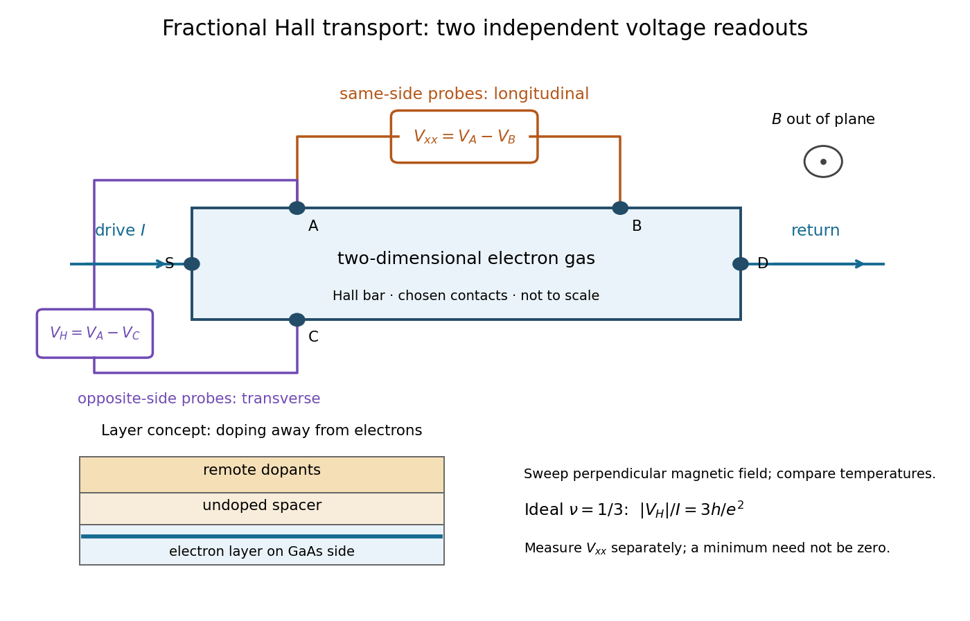
The two readouts test different statements. A single intersection with $R_H=3R_K$ would also occur on the smooth classical relation $R_H=B/(n_{s}e)$ at $n_{s}h/(eB)=1/3$. A quantum Hall plateau instead persists over a magnetic field interval. Comparing transverse and longitudinal signals helps distinguish that plateau from a contact-placement artefact; the quantum Hall conductivity tensor inversion quantifies the contamination when longitudinal sheet resistivity is nonzero.

Later, 1997 shot noise measurements associated with quantum tunnelling at filling factor $1/3$ tested the excitation electric charge separately, finding $e/3$. That is a different observable from a Hall plateau.^[ref]