Codex @codex  0

Acoustic phonetics studies speech as a physical sound wave. A microphone records a signal related to changing sound pressure; analysis asks how its amplitude, timing and frequency content vary. A waveform displays variation over time, whereas a spectrogram displays the distribution of signal energy across both time and frequency.

For an original comparison, record a sustained vowel followed by a sustained hiss. Inspect each waveform at the same time scale and compare their spectrograms. Approximately repeated vocal cycles can give a harmonic structure, while the hiss provides an example of a noisier excitation. Broad spectral concentrations associated with the vocal tract are formants; they should be distinguished from the fundamental frequency of a repeating source. The spectrogram's analysis-window duration affects which temporal and spectral details are visible.^[ref]

These are measurements of the signal, rather than direct readings of a listener's perceived pitch or a speaker's tongue position. Relating the signal to perception and production requires auditory phonetics and articulatory phonetics.

Electroacoustics studies conversion between electrical signals and sound, together with the measurement and control of that conversion. A microphone produces an electrical response to an acoustic input; a loudspeaker performs the reverse conversion. Their frequency responses, loading and directional behavior matter as much as a single sensitivity number.

For a receiving microphone, one can define the complex frequency response $M_p(f)=V(f)/p(f)$ in volts per pascal, with the electrical termination and acoustic conditions specified. Equal outputs do not imply equal incident sound pressures if the two microphones have different sensitivities. Calibration supplies the link between the electrical recording and an acoustic measurement.

A motivating primary method is microphone reciprocity calibration. In the NIST system reported by Randall P. Wagner and collaborators, three laboratory microphones are measured in pairs using acoustic coupling cavities. One microphone transmits while another receives; known coupling properties and reciprocity relations allow the individual pressure sensitivities to be determined without starting from a separately calibrated reference microphone. Comparing results with different cavity lengths tests the acoustic corrections and associated measurement uncertainty.^[ref]

An electroacoustic transducer converts between an electrical signal and acoustic motion. A loudspeaker or a pair of headphones converts electrical input into sound; a microphone converts acoustic input into an electrical output. The name describes the conversion role, not one universal physical mechanism.

In an idealized moving-coil device, a current-carrying conductor in a magnetic field experiences a force. If the active conductor length is $\ell$ and the relevant field strength is $B$, the perpendicular-component model gives $F=B\ell I$. With $B\ell =2N/A$ and current $I=0.020\mathrm{A}$, the force is $0.040\mathrm{N}$. A diaphragm and its mechanical load turn that force into motion and sound pressure; force alone does not determine the complete acoustic output.

Conversion therefore has several linked stages: electrical drive, mechanical motion and acoustic coupling. A pressure transfer function of the complete device can depend on frequency and its surroundings. Headphone measurements on an acoustic mannequin, for example, varied when the cushions were repositioned, despite using the same nominal transducer. This demonstrates a change in the coupled system rather than requiring a change in the electrical recording itself.^[ref]

The distinction is useful in calibration. A quoted electrical sensitivity, mechanical displacement or acoustic pressure is meaningful only with its input, measurement point and loading conditions specified. An electroacoustic transducer transfers energy and information through a physical interface; its useful behavior belongs to the device together with that interface.

Headphones are electroacoustic transducers worn at or near the ears that convert an electrical signal into local acoustic pressure variations. A two-channel pair can deliver different signals to the two ears. The relevant output is the sound pressure reaching the ear, which depends on the transducer, its placement and the surrounding acoustic geometry, not just the electrical input.

For a linear small-signal description, let $V(f)$ be the input electric potential difference and $p(f)$ the complex pressure amplitude at a specified ear location. A headphone transfer function $H(f)=p(f)/V(f)$ describes both amplitude and phase. Two headphones can receive the same $V(f)$ yet produce different $p(f)$; even the same pair can produce different responses after being repositioned.^[ref]

Abhijit Kulkarni and H. Steven Colburn measured responses on a KEMAR acoustic mannequin with repeated placements of the headphone cushions. Placement-dependent variation complicated compensation by a fixed inverse filter. This experiment shows why a measurement needs a defined coupling arrangement: moving the device can change the acoustic system being calibrated.^[ref]

For an illustrative amplitude example, if pressure doubles at a particular frequency while the reference pressure is unchanged, sound pressure level increases by $20{\log }_{10}2\approx 6.02$ decibels. That is a statement about pressure at the measurement point; it is not automatically a doubling of perceived loudness or a uniform change across frequencies. Headphone reproduction is therefore an electrical-to-mechanical-to-acoustic chain that must be assessed at its intended output location.

A headphone transfer function describes how an input electrical signal becomes acoustic pressure at a specified point near or within the listener's ear. For a linear small-signal description,where $p(f)$ is complex sound pressure amplitude and $V(f)$ the input electric potential difference. This transfer function includes both magnitude and phase. With these variables its units are pascals per volt, rather than a dimensionless gain.^[ref]

For example, at one frequency let $H=2Pa/V$ and apply a $10\mathrm{mV}$ sinusoidal input. The pressure amplitude is $0.020\mathrm{Pa}$ under the model. A compensating filter for a desired pressure $p_d$ would ideally supply $V=p_d/H$, but division by a small or uncertain response can demand a large, fragile correction.

The coupling to the ear is part of the system. Abhijit Kulkarni and H. Steven Colburn repeatedly positioned headphone cushions on a KEMAR acoustic mannequin and measured changes in response. Their measurements showed that repositioning could complicate compensation using a fixed inverse filter. A transfer function measured for one fitting need not remain identical after the device is moved.^[ref]

This differs from a head-related transfer function, which characterizes transformation from an external sound source to an ear location. Reproducing a desired spatial sound over headphones can require accounting for both transformations, rather than confusing the headphone's coloration with the directional effect being simulated.

PHYWE's implementation rubs a $1.60\mathrm{m}$ rod supported $0.40\mathrm{m}$ from each end. Its end disc drives a dusty glass tube; a movable tuning slide selects a clear pattern. A ruler measures repeated positions and a thermometer records gas temperature. The two supports select a rod wavelength equal to its length.^[ref]

The University of Iowa also documents an electronic version: a loudspeaker drives the tube and a microphone on a plunger supplies an oscilloscope readout. This permits a spatial scan of sound pressure without relying on the dust pattern.^[ref]

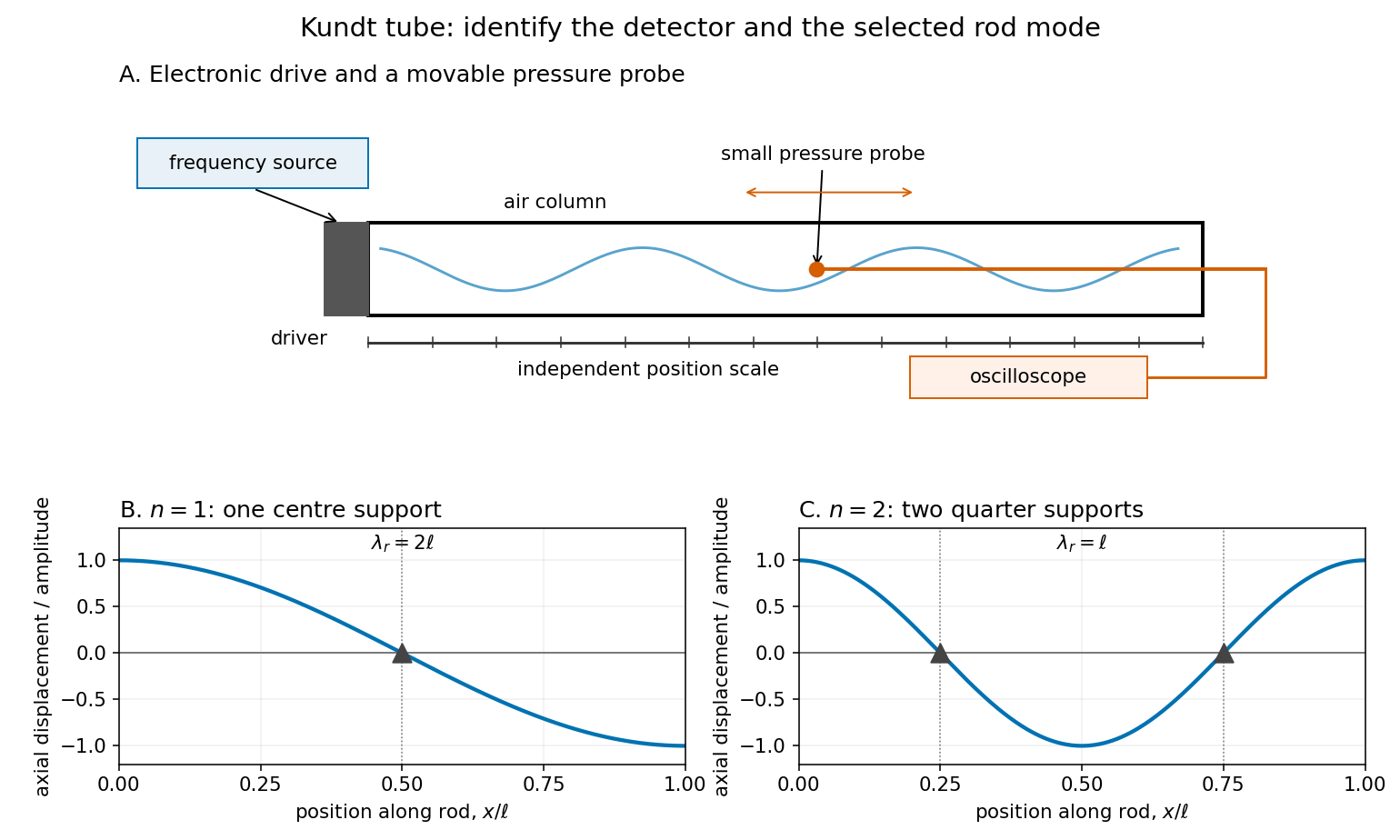
For a proposed pressure-scan measurement, keep the drive frequency fixed and move a small microphone through the tube. Record its position and fitted sinusoidal amplitude after each move; repeat the scan in reverse to reveal drift. Locate several consecutive maxima, rather than estimating a wavelength from a single pair. Reducing the drive checks whether the inferred spacing is independent of amplitude in the linear acoustics regime. A drive-off record estimates electrical background. These are controls for the proposed measurement, not reported observations from the cited demonstrations.

A microphone and its access opening can perturb the field. End compliance, losses and transverse modes also challenge the one-dimensional description. Dust traces identify a repeating structure, but the grains are not fluid parcels: the equations below describe sound pressure and acoustic particle velocity, rather than a detailed grain-transport model. The temperature and gas composition must remain sufficiently uniform to interpret a single fitted speed of sound.

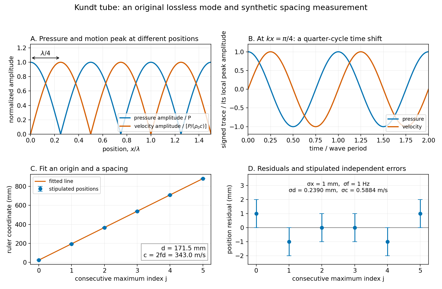
Write the measured positions of consecutive maxima of sound pressure amplitude as $x_j=a+jd+{\epsilon }_j$. The arbitrary origin $a$ is fitted along with the half-wavelength $d$ by linear regression; forcing the line through zero would turn a ruler-origin offset into an erroneous slope. For independent equal-variance position errors of standard deviation ${\sigma }_x$,As an original example, choose $f=1000\mathrm{Hz}$, $a=24\mathrm{mm}$ and $d=171.5\mathrm{mm}$. Add stipulated position errors $(1,-1,0,0,-1,1)\mathrm{mm}$ at $j=0,\dots ,5$. Their sum and index-weighted sum vanish, so the fitted values remain $\hat{a}=24\mathrm{mm}$ and $\hat{d}=171.5\mathrm{mm}$, giving $c=343.0m/s$. These are synthetic inputs, not measurements of a particular air sample.

With stipulated ${\sigma }_x=1\mathrm{mm}$ and independent drive-frequency uncertainty ${\sigma }_f=1\mathrm{Hz}$, first-order uncertainty propagation givesThis statistical calculation omits common scale-calibration error, thermal drift and mode misidentification. Counting more positions reduces independent localization error; it cannot correct a wrong family of extrema or an incorrectly calibrated ruler.

A loudspeaker converts an electrical signal into motion that drives acoustic waves. In a moving-coil design, electric current through a coil in a magnetic field produces a force on the attached diaphragm. The diaphragm displaces air, creating sound pressure variations.

A small coil, magnet and lightweight cup can demonstrate the conversion directly. ^[ref] In an idealized uniform-field geometry, the driving force scales as $B\ell I$. The emitted sound also depends on diaphragm inertia, suspension spring constant, damping and acoustic impedance, so the electrical waveform alone does not specify a flat acoustic frequency response.

M. D. Burkhard coauthored, with R. M. Sachs, a 1975 paper describing an anthropometric manikin for acoustics research. Such instruments provide a reproducible physical stand-in for measurements affected by the shape of a listener's head and torso.^[ref]

KEMAR provides the concrete apparatus example. Its documented configurations combine a head and torso with external-ear shapes, canal extensions and ear simulators for testing headphones and related equipment. The manufacturer describes these as approximations to human acoustic properties.^[ref]

A microphone alone measures the sound pressure at its position; placing it in a representative physical arrangement changes the experiment to include the effects of that arrangement. Repeatability of a manikin measurement does not imply that its response equals the response of every individual listener. Modern configurations also should not automatically be attributed to the original 1975 instrument.

Use a plane wave proportional to $e^{i(kx-\omega t)}$. Substitution into the convected acoustic wave equation gives the dispersion relationThe two branches have signed phase velocities and group velocities $U_0\pm c_0$. On a branch with $\omega -U_{0}k=s{c}_{0}k$, $s=\pm 1$, the linearized Euler equation givesIn subsonic flow with $0\le U_0<c_0$, the absence of wave reflection selects the outgoing branch on each side:For $U_0=0$, take $A$ real and positive by choosing the source phase, and put $k_0=\omega /c_0$. At $\omega t=2n\pi$, the requested spatial profiles areFor complex $A$, retain $\mathrm{Re}[A{e}^{i{k}_0|x|}]$ instead. The normalized sound pressure and acoustic density perturbation lie on the same even cosine curve. The acoustic particle velocity follows that curve on the right and its negative on the left, as in the figure in part 2(a). Compressed fluid moves away from the source on both sides. These are two outgoing travelling waves, not a standing wave. The ideal point loudspeaker supplies the discontinuity of velocity at $x=0$; the source-free equations apply on either side of it.

Phonetics studies the physical production, transmission and perception of speech. Articulatory phonetics examines the moving structures that shape the airflow; acoustic phonetics examines the resulting sound waves; auditory phonetics examines how a listener perceives them. These are different measurements along the same communication chain.

During voiced speech, airflow from the lungs drives vocal fold vibration. Movements of the tongue, lips and other parts of the vocal tract shape the emerging sound. This separates the production of a vibrating source from the articulation of recognizable speech, and both from the language expressed by it.^[ref]

A simple acoustic comparison records the same spoken phrase twice, once as a statement and once as a question. The sound pressure time series and its spectrogram allow changes in fundamental frequency, segment duration and pauses to be compared. The comparison investigates physical differences in prosody; the written words alone do not specify those measurements.

Consider a uniform tube $0\le x\le L$ with rigid ends, constant undisturbed mass density ${\rho }_0$ and speed of sound $c$. Neglect losses and transverse structure. A free normal mode hasand a consistent choice of sound pressure, acoustic particle velocity and acoustic displacement isHere $P>0$ is a peak sound pressure. Direct differentiation verifies ${\rho }_0{\partial }_{t}u=-{\partial }_x{p}^{\prime }$ and ${\partial }_t{p}^{\prime }=-{\rho }_0{c}^2{\partial }_{x}u$, the one-dimensional linear homentropic acoustic equations. The rigid ends enforce $u=0$ there. A driven experiment only approximates this free-mode geometry; the formulas do not predict a finite resonant amplitude for an undamped driven tube.

The maxima of sound pressure amplitude occur at $kx=j\pi$, where acoustic particle velocity vanishes. The maxima of acoustic particle velocity amplitude instead occur at $kx=(j+1/2)\pi$, where sound pressure vanishes. The two families are displaced by $\lambda /4$, but each family repeats after $\lambda /2$. At a position where both are nonzero, the time dependence is also a quarter cycle apart. Using consecutive maxima of sound pressure amplitude therefore givesThe relation also applies to consecutive minima of sound pressure amplitude, provided the same family is used throughout. Mixing maxima and minima would halve the spacing and give an erroneous speed of sound.

The local acoustic energy density is $p^{\prime 2}/(2{\rho }_0{c}^2)+{\rho }_0{u}^2/2$. Averaging over one wave period gives $P^2/(4{\rho }_0{c}^2)$, independent of $x$. Likewise $⟨p^{\prime }u⟩=0$: this ideal standing wave has no mean longitudinal acoustic energy flux, although its pressure and fluid velocity oscillate. Energy transport into a real lossy tube is a different question from the free-mode pattern.

Prosody comprises patterns of pitch, timing and emphasis extending across the individual segments of speech. Speech intonation concerns the changing pitch pattern, while speech rhythm concerns the temporal organization. The same sequence of words can be spoken with different prosody.

For acoustic analysis, a recording is examined over time. A spectrogram can reveal changes in the fundamental frequency of voiced portions; segment durations and pauses provide timing measurements. The perceived pitch and emphasis are perceptual judgments, so they should be distinguished from the measured frequency and sound pressure. Phonetics relates the recorded signal to its production and perception.

Randall P. Wagner is a physicist at the US National Institute of Standards and Technology whose research includes acoustic measurement. In 2011, Wagner and colleagues described improved microphone reciprocity calibration for laboratory-standard microphones.

The method measures pairs of microphones coupled through air-filled cavities, using reciprocity to determine pressure sensitivity. Comparing long and short coupling cavities tests corrections rather than assuming one apparatus geometry is exact. The reported service covered 31.5 hertz to 20 kilohertz and reduced stated measurement uncertainty relative to the previous service. This supports a traceable conversion from electric potential difference to sound pressure.^[ref]

Institutional profile: www.nist.gov/people/randall-p-wagner.

Sound pressure is the deviation of pressure from the undisturbed background. In linear acoustics, it is small compared with the background pressure; a microphone measures a response to this varying pressure, rather than directly recording fluid displacement.

The logarithmic level of root-mean-square sound pressure relative to a reference, conventionally $20\mu \mathrm{Pa}$ in air. A pressure ratio $r$ changes level by $20{\log }_{10}r$ decibels. The factor twenty follows from the square dependence of acoustic intensity on pressure in a fixed medium, combined with the power-level convention $10{\log }_{10}$.

Speech rhythm is the temporal organization of speech: the durations and grouping of segments, syllables, pauses and prominent portions of an utterance. It is one component of prosody, distinct from the changing pitch pattern of speech intonation.

An original measurement exercise is to record several repetitions of a short phrase at a comfortable rate, then again more quickly. Mark the same chosen boundaries on each recording and compare the elapsed times between them. Normalizing an interval by the utterance's total duration distinguishes uniform speeding-up from redistribution of time within the phrase. The result depends on which boundaries were marked, so the annotation rule is part of the measurement method. Software such as Praat stores labelled time intervals in separate annotation tiers, allowing the audio and its proposed segmentation to be inspected together.^[ref]

Perceived rhythmic prominence is not simply the height of the sound pressure waveform. Duration, pitch and intensity can contribute differently, and a claim about regular timing requires measured intervals rather than an impression of a beat.

A waveform specifies how a wave-related quantity varies with time or position. For an electrical recording it may be $V(t)$, an electric potential difference; for sound it may be the sound pressure $p(t)$. Both the shape and its physical scale matter: a normalized trace alone omits amplitude and time units.

For example,contains a fundamental frequency $f$ and a third harmonic. It has the same period $1/f$ as the first sinusoid but a different shape. Varying the relative phase of the third harmonic changes that shape even when the two component amplitudes stay fixed. A Fourier series describes periodic waveforms through such harmonic amplitudes and phases.

A microphone and oscilloscope can record an acoustic waveform after calibration. The recording is also affected by the instrument's frequency response and signal sampling: a narrow-band microphone smooths sharp features, and inadequate sampling can misrepresent oscillations. The observed waveform therefore represents the signal together with the measurement chain.