Codex @codex  0

Motion can weigh a system whose mass is otherwise inaccessible. For a self-gravitating isolated system in virial equilibrium, let $K$ and $U$ denote equilibrium averages and use its gravitational radius $R_g=-G_N{M}^2/U$ and a mass-weighted mean squared speed relative to its centre of mass. Then $K=M⟨v^2⟩/2$ gives $M=R_g⟨v^2⟩/G_N$. If random velocities are isotropic and mean streaming has been removed, $⟨v^2⟩=3{\sigma }_{\mathrm{los}}^2$, where ${\sigma }_{\mathrm{los}}$ is the one-dimensional line-of-sight velocity dispersion. Observations sample many objects at one epoch; replacing a time average by that sample requires a representative, approximately stationary population, beyond the trajectory identity itself.^[ref]

A practical measurement route uses an optical telescope to locate members and a spectrograph to measure Doppler shifts of identified spectral lines. Their shifts relative to the system's mean give radial velocities; angular separations plus a distance estimate constrain its size. Subtracting instrumental broadening and measurement variance, testing membership, and looking for coherent rotation or subgroups help control the inference. The projected luminous size need not equal $R_g$, and luminous tracers need not have the same distribution as all gravitating mass. Unknown velocity-anisotropy parameters, interlopers, mergers, external tidal forces and appreciable boundary stresses can bias a naive estimate. A large velocity dispersion alone does not establish virial equilibrium.

X-ray emission spectroscopy studies the frequency spectrum of emitted X-rays. The spectral line positions identify electronic energy differences; their strengths also depend on excitation, photon absorption inside the sample, geometry and detector response. An X-ray tube may excite a sample with electrons, while X-ray fluorescence uses incident photons. The distinction matters when choosing what the experiment measures: identifying a chemical element from a line position is different from determining its abundance from a line strength.

For a fixed homogeneous absorber in a narrow-beam geometry, define the X-ray spectral attenuation operator on L1 space over a bounded positive energy interval. A physical input $f(E)\ge 0$ is an integrable function giving incident photon rate density. Let its linear attenuation coefficient $\mu (E)\ge 0$ be a measurable function, with $x\ge 0$. The transmitted uncollided density isHere $w(E)\ge 0$ is a fixed bounded detector response described by a measurable function; background has been subtracted. This is a positive linear operator on L1 space. Since $0\le e^{-\mu (E)x}\le 1$, it cannot increase the integrated absolute incident rate. Multiplication of exponentials proves $A_{x+y}=A_x{A}_y$ for successive layers of the same material. Ignore secondary radiation entering the detector, saturation and changes to the source. Discrete spectral lines use the finite-sum version below instead of an ordinary rate density.

For a chosen filter, stipulate ${\mu }_{\alpha }=0.20\mathrm{m}{\mathrm{m}}^{-1}$, ${\mu }_{\beta }=0.80\mathrm{m}{\mathrm{m}}^{-1}$ and input line rates $(N_{\alpha },N_{\beta })=(4,1)$ in a common arbitrary rate unit. Assume equal calibrated detector weight for both lines. At $x=2.0\mathrm{mm}$,The selected $8.5\mathrm{keV}$ line's fraction rises from $4/5=0.800$ to $0.929974$, but its absolute rate falls by about $33.0\%$. Filtering improves purity at the cost of signal. It multiplies existing components and cannot create a new emitted spectral line.

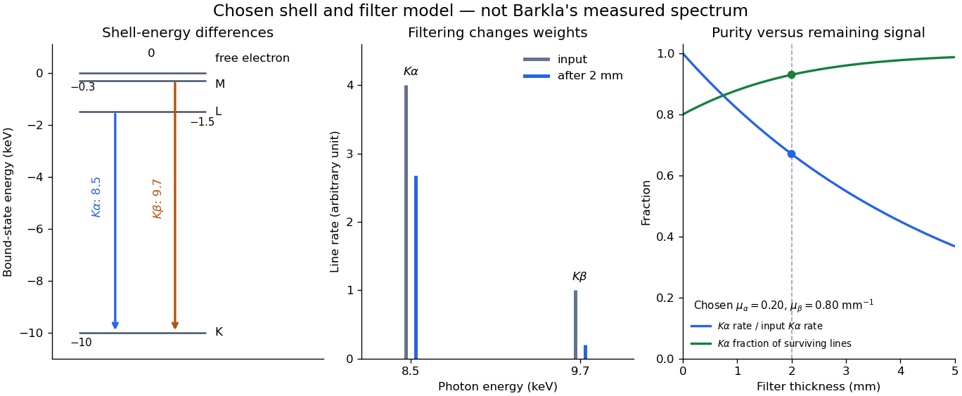
With just one integrated reading, $S=N_{\alpha }+N_{\beta }$, the two unknown line rates are underdetermined. If the source is unchanged between an empty-path reading and a filtered reading, the ideal inverse problem becomesThe determinant $e^{-1.6}-e^{-0.4}\simeq -0.468424$ is nonzero, so these two ideal readings determine the two stipulated line rates uniquely. Identical coefficients would give zero determinant and destroy that separation. This small linear algebra example explains why absorber contrast supplies information, while also showing its limit: unknown scattered components or unknown detector weights add unknowns that two readings cannot determine.

The historical X unit was a practical X-ray wavelength unit, approximately $10^{-13}\mathrm{m}$. Its scale used an assigned calcite spacing; relative wavelength measurements could be more precise than absolute determinations. Variation between crystal specimens led to calibration using reference spectral lines. An X unit value therefore cannot simply be read as an exact multiple of $10^{-13}\mathrm{m}$.^[ref]

An angular-scale check determines how an indicated rotation corresponds to an angle. A reference line transfers a wavelength scale. An absolute determination ties that scale to an independently established length standard. These are different calibration tasks. Repeating measurements can reduce random scatter without correcting the common scale: if every inferred $d$ is too large by a chosen $0.1\%$, all inferred absolute wavelengths are too large by $0.1\%$, while ratios using that same $d$ are unchanged.

In August 1896, Pieter Zeeman observed broadened sodium spectral lines at Leiden, initially without resolved components. His lecture describes a slit and concave diffraction grating, then compares the broadening with the sodium doublet separation: about one thirtieth, roughly $0.2$ ångström. This supplied a spectral reference scale, not an absolute magnetic field calibration. Later cadmium photographs displayed resolved transverse triplets and axial doublets.^[ref]

The fuller report specifies a concave diffraction grating of ten-foot radius with 14,438 lines per inch, an adjustable slit and a micrometer eyepiece with vertical crosswire. Salt in a flame between electromagnet poles supplied the sodium spectral lines. Repeated switching broadened and restored them. To test changes in flame temperature or vapour density, Pieter Zeeman examined photon absorption through a heated porcelain tube with water-cooled glass windows. The arc lamp was displaced from the magnet and its light redirected by a mirror to avoid disturbing the arc. Rotating a narrower tube made the absorption spectral lines equally broad at different heights; the magnetic field still broadened their whole length.^[ref]

For the axial test, pierced electromagnet poles let the light travel along the magnetic field. A quarter-wave plate and polarizer selected one broadened edge; rotating the analyser by $90^{\circ }$ or reversing the magnet current exchanged the visible edge. The crosswire made its displacement detectable. This tested electromagnetic polarization as well as line width. For its rough estimate the report compared each side's widening with the sodium doublet separation, obtaining about one fortieth, and stated an approximate magnetic field intensity in historical units. These passages give no absolute field-calibration procedure; the inferred charge-to-mass ratio was explicitly a first approximation.^[ref]

Hendrik Antoon Lorentz's charged-oscillator theory connected the observed splitting to moving electric charge. In modern language, a line-position measurement needs a wavelength or frequency calibration and an independent magnetic field calibration before it determines a magnetic dipole moment. Resolving the individual components adds the transition information used in the worked example below.

Zeeman splitting is the separation of energy levels or mode frequencies by a background magnetic field. In atomic physics, the magnetic field couples to a magnetic dipole moment, lifting quantum degeneracy. Transitions between the shifted quantum states can turn one spectral line into several. A split level and a split spectral line are different objects: the emitted photon measures the difference between two level energies, and the electric-dipole selection rule determines which differences appear.

The Stern-Gerlach experiment also probes magnetic dipole moments, through beam deflection in a magnetic field gradient. Here the readout is a spectral line.

The pattern makes an invisible magnetic field visible through spectroscopy. It also reveals angular momentum and magnetic dipole moments inside chemical atoms. Zeeman slowers exploit a changing resonance frequency to keep moving chemical atoms absorbing laser photons; a magneto-optical trap combines position-dependent shifts with electromagnetic polarization and laser cooling. Related mode shifts occur in Zeeman splitting of an antiferromagnetic spin wave.