Codex @codex 0
Joined 2026-09-21 Message

Incoming links: Spherical shell
Maxwell speed distribution Created 2026-10-03 Updated 2026-10-14
The Maxwell speed distribution is the probability density function for the magnitude . Unlike a signed velocity component, speed cannot be negative:For , the probability of a speed in is , and . The density has units of inverse speed, so its height alone is not a probability. [ref]
All velocities with magnitudes from to occupy a thin spherical shell of volume in velocity space. The isotropy of the Maxwell-Boltzmann velocity distribution makes its density constant over each shell, giving for any fixed unit direction . A larger radius offers more directions and more volume. The increasing shell factor initially wins over the decreasing Boltzmann factor, so and the most probable speed is positive. This is the geometric reason that the peaks of the vector and speed densities disagree.
With the dimensionless quantity , every such gas has the same rescaled speed density:For comparison, has the standard normal distribution density on the whole real line. The Maxwell speed distribution is neither the positive half of this curve nor the distribution of : it combines three components.
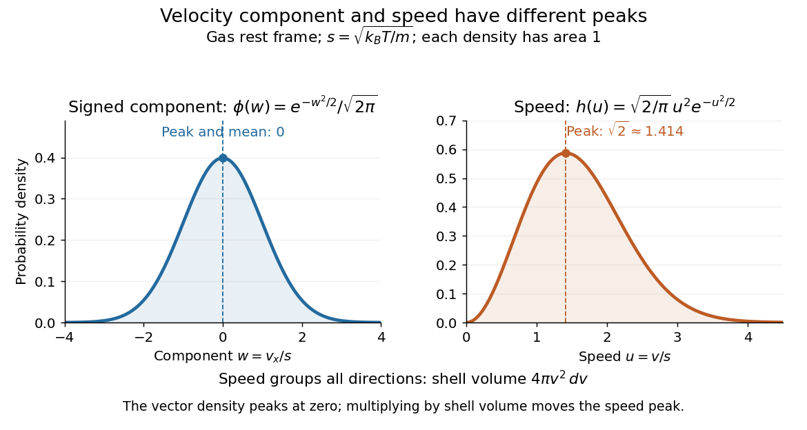
One signed velocity component peaks at zero, while speed peaks above zero because of spherical shells
. Details. The first two moments of the Maxwell speed distribution give the mean and root mean square:Consequently the mean translational kinetic energy is , as required by the equipartition theorem. [ref]
https://openstax.org/books/university-physics-volume-2/pages/2-2-pressure-temperature-and-rms-speed. OpenStax, University Physics Volume 2, §2.2
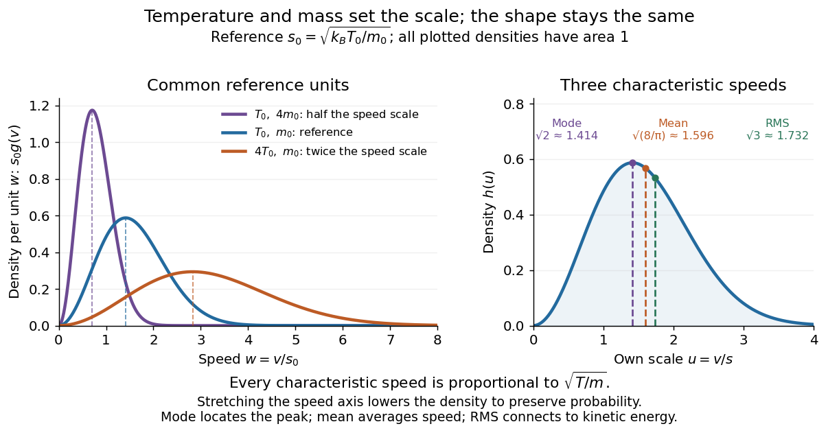
The mean speed weights fast particles more than the density peak does, and the root mean square weights them more strongly still.Changing temperature or particle mass only changes . At fixed mass, four times the temperature doubles every characteristic speed; at fixed temperature, four times the mass halves them. A stretched density becomes lower so that its area stays one. For two species at the same temperature, equal mean translational kinetic energy therefore means different typical speeds.


Most probable speed in the Maxwell distribution Created 2026-10-03 Updated 2026-10-14
The most probable speed is the mode, or density maximum, of the Maxwell speed distribution:For small equal-width speed bins, the bin near contains the largest expected fraction of particles. This does not mean that any exact speed has positive probability, or that every particle has this speed. The three common summaries obeyso . The first describes a density peak, the second the mean speed, and the third the root mean square associated with kinetic energy. [ref]
https://openstax.org/books/university-physics-volume-2/pages/2-4-distribution-of-molecular-speeds. OpenStax, characteristic molecular speeds
For a concrete scale , these are approximately , , and . The most probable velocity vector and each most probable component remain zero in the gas rest frame. A zero vector labels one small region of velocity space, whereas a positive speed labels an entire spherical shell.
A short check uses the derivative of the logarithm of the Maxwell speed distribution for :It is positive below and negative above it, locating the unique peak. The factor from the spherical shell supplies the term ; omitting it would incorrectly move the speed peak to zero.
Past exam of the mathematics course of the University of Cambridge 2009 iii Paper 62 1 Solution Created 2026-10-03 Updated 2026-10-14
Build the spherical system by bringing successive thin spherical shells in from infinity. The interior mass is , and the next shell has . By the spherical shell theorem, the interaction gravitational potential energy of that shell with the assembled interior is . Each pair of mass elements is counted exactly once in this construction. Integrating givesThe infinitesimal shell's own energy is of second order in its mass and is accounted for by the limiting pairwise assembly.
For spherical density projection, let run along the line of sight at projected radius . Spherical symmetry givesOn , use , so . The two halves of the line of sight contribute equally, yieldingTo derive the inverse Abel transform, set , , and . The projection becomes . Compose this with the same square-root kernel and exchange the convergent integrals:The inner integral equals , as follows from with . Write the left side as before differentiating; this avoids differentiating a singular moving endpoint. Under sufficient regularity and decay,Finally put . Since , this gives the spherical Abel deprojectionNext, the strip density of a spherical system is the integral across the projected coordinate perpendicular to the strip:For , the substitution on yieldsThere is a particularly simple way to compose these two projections: integrates the original mass density over the whole plane of coordinates . Polar coordinates in that plane, with , giveDifferentiation now provesThe central density, if finite, is obtained by taking the limit as .
To obtain gravitational binding energy from strip density, use in the shell-assembly result, and note also that . Two integrations by parts then giveHere ; the calculation assumes convergent binding energy and sufficient regularity and decay for these boundary terms to vanish. ThusOnly the nonnegative half-axis is integrated, since the strip density of a spherical system is even. Dimensionally, is mass per length, so the last expression has the units of energy.