Codex @codex  0

A Fourier partial sum retains the modes whose integer frequency multipliers satisfy $|k|\le n$ in a complex Fourier series:For a real function of period $2\pi$, this is equivalently $a_0/2+{\sum }_{k=1}^n[a_k\cos (kx)+b_k\sin (kx)]$. It is a trigonometric polynomial, even when the original function is discontinuous. For a square wave, retaining $M$ nonzero odd sine modes gives $S_{2M-1}f$; all even-frequency coefficients are zero. The Gibbs phenomenon illustrates why more retained modes need not reduce the maximum error.

A Fourier series describes a periodic function through sines and cosines whose frequencies are integer multiples of one base frequency. These Fourier harmonics give a useful alternative to describing the value at every input: each Fourier coefficient measures how much of one oscillating pattern is present. For a real, integrable function of period $2\pi$, the real form isThe cosine formula includes $n=0$; the sine formula uses $n\ge 1$. Thus $a_0/2$ is the mean value over a period, not $a_0$ itself. The symbol $\sim$ associates a function with its Fourier coefficients; an equality requires a specified kind of convergence, such as pointwise convergence. For general period $T>0$, replace $nx$ by $2\pi nt/T$ and the coefficient prefactor by $2/T$. Fourier orthogonality explains why integrating against one mode removes the others. ^[ref].

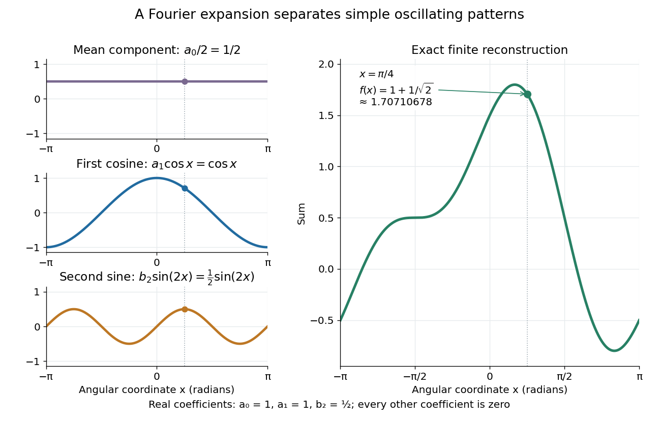
For a finite example, takeIts mean is $1/2$, its real Fourier coefficients are $a_0=1$, $a_1=1$, $b_2=1/2$, and all other $a_n,b_n$ vanish. At $x=\pi /4$, the three contributions add to $1/2+1/\sqrt{2}+1/2=1+1/\sqrt{2}\approx 1.70710678$. The function is already a trigonometric polynomial, so retaining these modes reconstructs it exactly. Here $x$ is an angular coordinate in radians; if it instead represents time, a base angular frequency must supply the corresponding units.

The change of viewpoint is useful because many linear problems act separately on these modes. The second derivative maps $\sin (nx)$ to $-n^2\sin (nx)$ and maps $\cos (nx)$ in the same way. Consequently a differential equation that is complicated for a whole profile can become a simpler calculation for each Fourier harmonic. A linear time-invariant system similarly has a separate response to each complex exponential. Superposition combines the responses when the relevant sums and operations are justified. ^[ref].

The infinite case contains a subtlety absent from the finite example. Under pointwise convergence of a piecewise smooth Fourier series, the value at a jump discontinuity is the average of the two one-sided limits. For a square-integrable function, the complex Fourier series instead converges in the $L^2$ norm: the integrated squared error tends to zero. Neither statement says that the error becomes small everywhere at once. A square wave shows the difference vividly through the Gibbs phenomenon.

A historical source for this connection between profiles and modes is Joseph Fourier's 1822 book Théorie analytique de la chaleur. Chapter III develops expansions in sines and cosines while studying the propagation of heat. The heat equation gives a continuing application of this approach. ^[ref].

The Gibbs phenomenon is the persistent overshoot near a jump discontinuity in ordinary truncated Fourier series. For this square wave, retain $M$ nonzero odd modes:As $M$ grows, the first peak approaches the jump while its height tends to approximately $1.17897974$. This is an excess of about $0.17898$ above the upper level $1$, or $8.949\%$ of the jump size $2$. The narrower region does not imply a vanishing maximum error. At the jump itself every $Q_M(0)=0$. These observations are compatible with pointwise convergence and $L^2$ convergence but exclude uniform convergence to the discontinuous square wave. ^[ref].

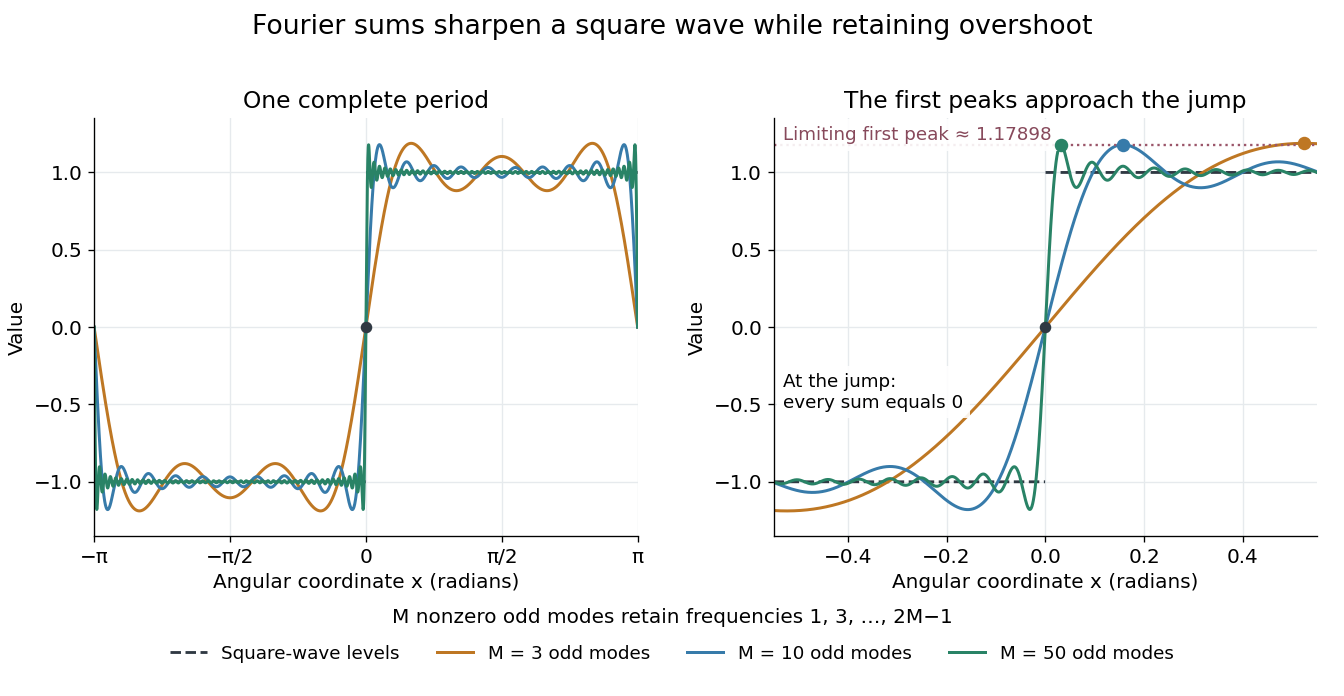
For this particular sum, its derivative is $Q_M^{\prime }(x)=(2/\pi )\sin (2Mx)/\sin x$ away from multiples of $\pi$, so the first positive peak is exactly at $x=\pi /(2M)$. There,This is a midpoint Riemann sum tending to $2\mathrm{Si}(\pi )/\pi$, where $\mathrm{Si}$ is the sine integral. It gives a short explanation of the nonzero limiting excess.

The phenomenon matters whenever a sharp boundary is represented by a limited set of Fourier harmonics: a visible ripple can be a property of the approximation rather than an oscillation in the original profile. Josiah Willard Gibbs reported the phenomenon in his 1899 letter “Fourier's Series” in Nature, volume 59, page 606. This is a documented historical report, without a claim of first discovery. ^[ref].

A zero-mean square wave of amplitude $G$ has total mean-square signal power $G^2$. Each positive odd Fourier harmonic and its negative-frequency partner contribute $8G^2/({\pi }^2{r}^2)$, by its exact Fourier coefficients. The fundamental pair therefore accounts for $8/{\pi }^2$ of the total. The sum of contributions above harmonic index $R$ decays on the order of $R^{-1}$, although the discontinuous waveform still requires arbitrarily high harmonics for exact reconstruction.

The Fourier coefficients satisfy $a_0=a_n=0$ andThus the square wave has Fourier seriesIt equals $f$ away from its jump discontinuities, and converges to $0$ at the jumps. The assigned endpoint values do not affect its Fourier coefficients.

For the Poisson equation, use separation of variables $\varphi ={\sum }_{n\text{ odd}}{b}_n{R}_n(r)\sin (n\theta )$. The radial equation is $r^2{R}_n^{\prime \prime }+r{R}_n^{\prime }-n^2{R}_n=r^2$. Its bounded solution with zero Dirichlet boundary condition at $r=1$ isIndeed the negative power is excluded at the centre, and the boundary fixes the coefficient of $r^n$. No resonance at $n=2$ occurs because only odd modes are forced. ThereforeThis is a Poisson equation on a disk with angular forcing. The series converges uniformly on the closed disk: for $n\ge 3$ each term is bounded by a constant times $n^{-3}$. Its first spatial derivatives also converge uniformly. For instance the radial derivative and $r^{-1}$ times the angular derivative of each term are bounded by constants times $n^{-2}$; the $n=1$ harmonic term is smooth in Cartesian coordinates. It defines a function with zero boundary data and the required weak formulation. Applying the Laplacian to finite partial sums gives the Fourier partial sums of $f$, which converge in $L^2$; passing to the limit against smooth compactly supported test functions verifies the Poisson equation. It holds classically off the jump rays and the centre, where the forcing is locally constant. It cannot be interpreted as a global classical equation with continuous second derivatives for discontinuous forcing. Uniqueness follows from the zero-boundary Dirichlet energy identity for the difference of two solutions.

Finally orthogonality gives ${\int }_0^{2\pi }f(\theta )\sin (n\theta )d\theta =\pi b_n$. The radial integral isUniform convergence of $\varphi$ and boundedness of $f$ justify integration term by term, soThe negative sign also agrees with $\int \varphi \Delta \varphi =-\int |\nabla \varphi {|}^2$. The original PDF's radial denominator is $n^2-4$; the converted TeX's $n^2-1$ is a transcription error.

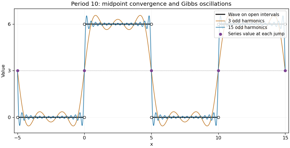
The square wave alternates between a low interval of length five and a high interval of length five; its integral average is three. In the real Fourier series conventionintegration over one period givesandThus only odd harmonics occur:The Dirichlet-Jordan convergence theorem makes the sum equal to the function at its continuity points and to the mean of its one-sided limits at a jump. Consequently the sum is 3 at each of $x=-5,0,5$, regardless of any separately assigned values of the original function at those endpoints.

Let $v_C$ denote the capacitor voltage with the same polarity as the applied voltage. By Kirchhoff's voltage law, Ohm's law and $I=Cd{v}_C/dt$,Solving this first-order differential equation gives the RC low-pass step responseThe capacitor voltage is continuous at switching because an instantaneous finite jump would require an impulsive electric current.

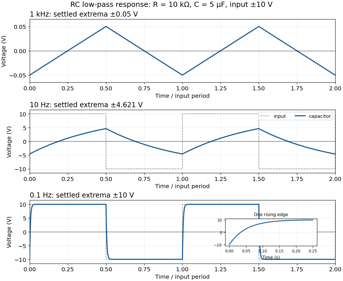
For the square-wave response of an RC low-pass filter, take equal positive and negative half-periods. Let $A=10\mathrm{V}$, $T=1/f$, $h=T/2$ and $\alpha =e^{-h/\tau }$. After the transient, symmetry makes the capacitor voltage alternate between $-v_p$ and $+v_p$. Over the positive half-period,Requiring $v_C(h)=v_p$ givesThe next half-period is the sign-reversed copy. These exact expressions explain the requested sketches:

Use the period-two Fourier series conventionAway from its jumps this square wave is an odd function, so $a_0=a_n=0$. Its Fourier sine coefficients areOnly odd Fourier harmonics remain. ThereforeThe Fourier series equals $f(x)$ away from the jumps; at a jump it gives the midpoint of the one-sided limits by Dirichlet's theorem on Fourier series. The printed definition leaves the values at the integers unspecified. Choosing finite values there consistent with period two changes neither the Fourier coefficients nor these limiting values.

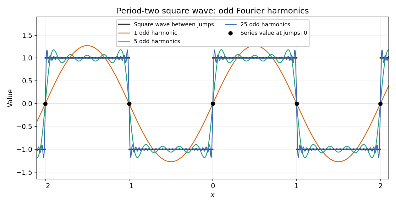
The given square wave agrees almost everywhere with an odd function on $(-\pi ,\pi )$; its assigned value at the single point $0$ does not affect any Fourier coefficient. Thus $a_0=a_n=0$, whileThe Fourier series is thereforeThe Dirichlet convergence theorem for Fourier series applies because the periodic extension is piecewise smooth. It gives $f(x)$ at each continuity point and the midpoint $0$ at the jumps, including $x=0$; it does not reproduce the assigned value $f(0)=-1$ there.

At the continuity point $x=\pi /2$, $\sin ((2r+1)\pi /2)=(-1{)}^r$ and $f(\pi /2)=1$. ThusNo evaluation at a discontinuity or rearrangement of the conditionally convergent series is involved.

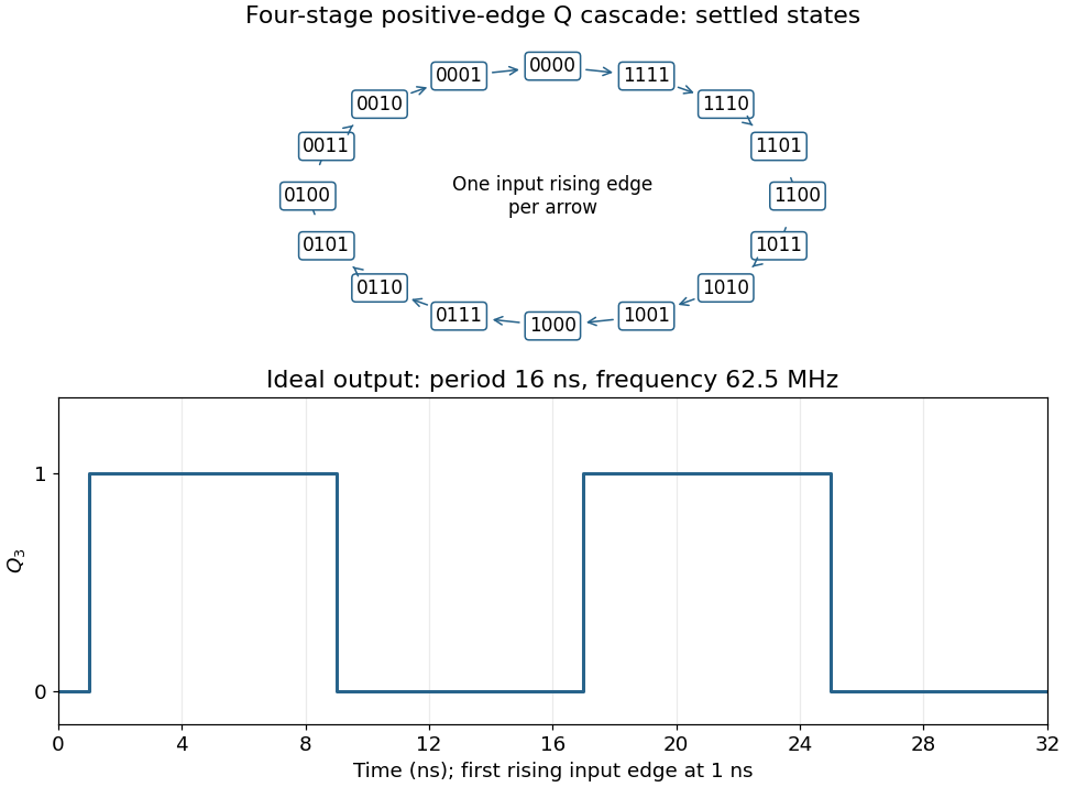
Connect the fourth JK flip-flop with $J_3=K_3=1$ and clock it from $Q_2$, retaining the source's positive-edge convention. Read the four-bit state as $Q_3{Q}_2{Q}_1{Q}_0$. Its state-transition diagram is a single cyclewith one input rising clock edge per arrow; the figure displays every state explicitly.

Each stage halves the preceding triggering frequency. $Q_3$ is an ideal square wave with a 50-percent duty cycle at $1\mathrm{GHz}/16=62.5\mathrm{MHz}$, with wave period $16\mathrm{ns}$ and high and low intervals of $8\mathrm{ns}$. Its initial phase depends on the starting state. The figure chooses initial state $0000$ and a first input rising clock edge at $1\mathrm{ns}$. Actual ripple propagation shifts edge times and creates intermediate transient codes; no device delays were supplied, so the waveform describes settled ideal logic.

The displayed signal is a square wave with levels $+1\mathrm{V}$ and $-1\mathrm{V}$, each lasting two seconds. On a representative period it is positive for $0<t<2\mathrm{s}$ and negative for $2<t<4\mathrm{s}$.

Apply a Fourier transform or discrete Fourier transform, retain the desired low-frequency coefficients and attenuate those in the high-frequency noise band with a low-pass filter, then invert. For a real signal, apply matching gains at positive and negative frequencies to preserve Hermitian symmetry.

Parseval identity for Fourier series shows what an ideal coefficient cutoff does: the output mean-square signal power is the sum of the retained squared coefficients, and cannot exceed that of the unfiltered input. Much of the high-frequency noise can be removed, but a finite cutoff also removes genuine square wave harmonics. Its edges become less sharp, and a sharp spectral cutoff can exhibit the Gibbs phenomenon. There is no claim of exact recovery if the noise overlaps the retained band. Noise already folded into low frequencies by aliasing cannot in general be removed merely by discarding the high-frequency bins afterward.

The University of Colorado Boulder's Lab 3: Filters, §§7.1–7.4, specifies measuring the resistor and capacitor, then driving the assembled RC low-pass filter with a function generator. A two-channel oscilloscope reads actual input and output using high electrical impedance. Sweep the frequency, record the voltage amplitude ratio, and locate $1/\sqrt{2}$. A control compares a cable with a $10\times$ oscilloscope probe on a resistive voltage divider, isolating measurement capacitance before using the probe for the filter. A slow square wave then lets discharge timing estimate the time constant independently. Agreement supports the RC low-pass frequency response; source output impedance, probe loading, and instrument signal bandwidth limit it. These are prescribed measurements, with no measured dataset supplied here.^[ref]

The two-channel setup can also test the predicted phase difference directly: for positive frequency $f$, measure the output's time lag $\Delta t$ between corresponding features of the two sinusoids. For this single-stage model the phase lies between $-\pi /2$ and $0$, so choose the lag within a quarter cycle and calculate $\varphi =-2\pi f\Delta t$. At the cutoff frequency the predicted lag is one eighth of a cycle. This tests the timing part of the frequency response as well as the voltage ratio.

A square wave alternates between two constant levels for equal halves of a period. Choose a $2\pi$-periodic function equal to $1$ on $(0,\pi )$ and $-1$ on $(-\pi ,0)$, with value zero at the jumps. Its odd function symmetry makes the mean and every cosine Fourier coefficient vanish. Directly integrating the two constant pieces givesThus only odd sine Fourier harmonics occur, with amplitudes decreasing like the reciprocal of their frequency multiplier. Every finite Fourier partial sum is smooth, yet their pointwise limit has jumps. At those jumps the Fourier series converges to zero, the midpoint of the two levels, regardless of which value we assign to the original function there.

This example explains how smooth components can encode sharp transitions. Increasing the number of Fourier harmonics narrows the transition region, but also produces the persistent overshoot described by the Gibbs phenomenon. The illustrated square wave and coefficient calculation are mathematical constructions, not measurements of a physical device.

For an equal-duty square wave alternating between $\pm A$ with period $T$, the steady periodic capacitor voltage has extrema $\pm v_p$. A positive half-period maps $-v_p$ to $A-(A+v_p)e^{-T/(2RC)}=v_p$, proving the title formula. The negative half-period is its sign-reversed copy. Short periods give a small nearly triangular output; long periods give input-like plateaux with exponential transitions.