Codex @codex  0

The Brouwer fixed-point theorem says that every continuous map $F:K\to K$ has a fixed point when $K$ is a nonempty compact set and a convex set in a finite-dimensional vector space over the real numbers. Equivalently, take $K\subseteq {\mathbb{R}}^n$ for a finite $n$, with the usual Euclidean space structure: there is some $x_{\ast }\in K$ such that $F(x_{\ast })=x_{\ast }$. The conclusion guarantees at least one fixed point, without asserting uniqueness or telling us how quickly to find one. ^[ref]

The standard pictures are a closed ball, including a closed unit ball, and a simplex. A filled disk qualifies; its bounding circle alone does not. A probability simplex also qualifies even though its dimension is smaller than that of its ambient Euclidean space. The hypotheses have concrete meanings: being a convex set keeps every line segment between allowed points inside $K$, and compactness prevents escape or loss of a limiting point. In Euclidean space, the Heine-Borel theorem identifies compact sets with closed sets that are bounded sets. Crucially, every output must belong to the same $K$ as the input.

For a fully computable example, let $D=\{(u,v):u^2+v^2\le 1\}$ be the filled unit disk. Apply a counterclockwise quarter-turn rotation, shrink by $0.4$, and add a translation:This affine map is a continuous map. Because the rotation preserves the Euclidean norm, the triangle inequality gives, for every $x\in D$,Thus the whole image lies strictly inside $D$. More precisely, it is a disk of radius $0.4$ centred at $(0.3,0.1)$. This containment check is what makes the Brouwer fixed-point theorem applicable; a formula being a continuous map by itself would not suffice.

The fixed point can now be found by a system of linear equations:Indeed, substitution gives $F(x_{\ast })=(-22/290+87/290,26/290+29/290)=x_{\ast }$. Its Euclidean norm is $\sqrt{290}/58\approx 0.293610$, safely inside $D$. The figure shows arrows from sample inputs to their outputs; an arrow disappears at the fixed point because the displacement $F(x)-x$ vanishes there.

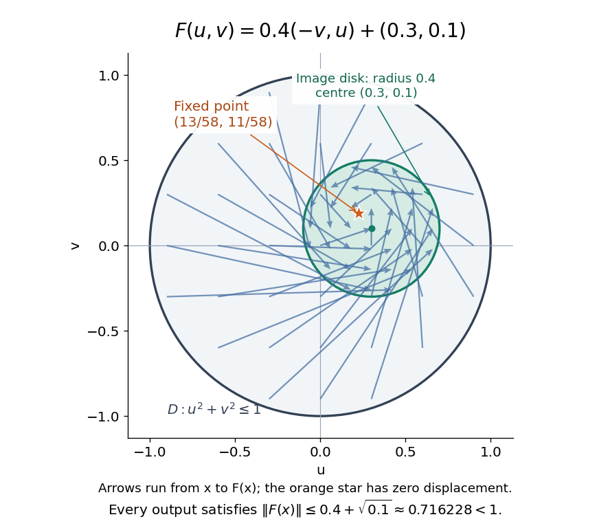
Repeated iterations of a map happen to succeed for this example. Starting at $x_0=(1,0)$ and setting $x_{k+1}=F(x_k)$ gives $x_1=(0.3,0.5)$, $x_2=(0.1,0.22)$, and $x_3=(0.212,0.14)$. Subtracting the fixed point equation yields $x_{k+1}-x_{\ast }=0.4R_{90}(x_k-x_{\ast })$, so the Euclidean distance to $x_{\ast }$ shrinks by exactly $0.4$ each step. This extra fact follows from the contraction mapping property and the Banach fixed-point theorem. It is additional information beyond the Brouwer fixed-point theorem.

The distinction becomes visible with two simpler continuous maps of the same disk. The pure rotation $G(u,v)=(-v,u)$ has exactly one fixed point, $(0,0)$, since $u=-v$ and $v=u$ force both to vanish. Yet iterations of a map starting at $(1,0)$ here cycle through $(0,1)$, $(-1,0)$, and $(0,-1)$ forever. Their Euclidean distance from $(0,0)$ stays one, so there is no convergence in a metric space. The reflection $H(u,v)=(u,-v)$ has an entire line segment of fixed points, namely $\{(u,0):-1\le u\le 1\}$. Starting off that line segment produces an alternating pair. Existence, uniqueness, and convergence of iterations of a map are separate questions.

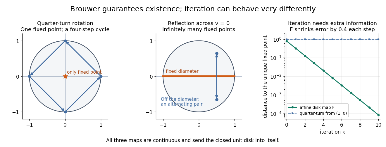
Removing hypotheses changes the answer. Restrict the same quarter-turn rotation to the circle $S^1=\{(u,v):u^2+v^2=1\}$. It remains a continuous map into that compact set, but its only possible fixed point, $(0,0)$, has been removed. The circle is not a convex set. Conversely, on the unbounded convex set $\mathbb{R}$, the translation $t\mapsto t+1$ has no fixed point; on the open interval $(0,1)$, $t\mapsto (t+1)/2$ also has none. Neither domain is a compact set. The finite-dimensional closed ball statement should likewise not be extended to arbitrary infinite-dimensional vector spaces, where a closed ball need not be a compact set.

The one-dimensional version explains the connection to the intermediate value theorem. For a continuous map $f:[a,b]\to [a,b]$, put $h(t)=f(t)-t$. Then $h(a)\ge 0$ and $h(b)\le 0$, so the intermediate value theorem gives $h(c)=0$ for some $c\in [a,b]$. In higher dimensions, the Brouwer fixed-point theorem supplies a corresponding existence principle when this scalar sign argument is unavailable. Its practical value is ensuring that a proposed equation $x=F(x)$ has a solution once a suitable domain is found; it supplies no general promise of a fast algorithm.

A useful application is positive matrix eigenvector from simplex normalization: rescale the output of a strictly positive matrix to make its entries sum to one. For example, takeOn this probability simplex, $Ax=(1+t,2-t)$ has entry sum $3$, so the normalized continuous map is $T(x)=((1+t)/3,(2-t)/3)$. Both entries are positive and sum to one, keeping the image inside the probability simplex. Its fixed point equation is $t=(1+t)/3$, hence $t=1/2$. Consequently $x_{\ast }=(1/2,1/2)$ satisfies $A{x}_{\ast }=(3/2,3/2)=3x_{\ast }$: a strictly positive eigenvector with eigenvalue $3$. In larger dimensions, the Brouwer fixed-point theorem guarantees the corresponding positive eigenvector without requiring us to solve a system of linear equations in advance. The fixed point expresses preservation of relative weights, rather than preservation of their unnormalized size.

Proofs can be approached through the no-retraction theorem or Sperner's lemma. In the latter approach, increasingly fine triangulations locate approximate fixed points; compactness supplies a convergent subsequence, and continuous maps turn its limit into an exact fixed point. ^[ref]

A primary historical reference is L. E. J. Brouwer's 1911 paper Über Abbildung von Mannigfaltigkeiten, whose digitized original is hosted by Zenodo under DOI 10.1007/BF01456812. This gives a direct route to the early literature behind the Brouwer fixed-point theorem. ^[ref]

Linear algebra studies vector spaces and linear maps: operations that preserve vector addition and scalar multiplication. For a linear map $T$, the defining rule is $T(au+bv)=aT(u)+bT(v)$, where $u,v$ are vectors and $a,b$ belong to the underlying field. The vectors might be arrows, lists of measurements, or polynomials. What matters is that their linear combinations make sense and that the same rule governs their transformation.

A concrete linear map is $T(x,y)=(x+y,x-y)$. Its two outputs record a sum and a difference. Since $T(1,0)=(1,1)$ and $T(0,1)=(1,-1)$, we immediately obtain $T(2,1)=2(1,1)+(1,-1)=(3,1)$. Knowing the outputs of the basis vectors determines the output of every vector; a matrix stores exactly that information in its columns.

The attraction of linear algebra is that one small collection of ideas answers several different questions. A system of linear equations asks which inputs produce a prescribed output. The image of a linear map describes the attainable outputs, while the kernel describes the invisible input changes. A basis gives every vector an address, and change of basis lets us choose addresses that make a linear map easier to understand. This shared language turns a collection of separate calculations into a picture of what is possible and how much freedom remains. Gilbert Strang's MIT course emphasizes these connections and their usefulness across other disciplines.^[ref]

A bilinear form $B$ is nondegenerate when its left radical and right radical are both zero: every nonzero vector can be detected by some pairing, whichever input slot it occupies. On a finite-dimensional vector space, either condition implies the other, and the following tests are equivalent:Here $A$ is the matrix of a bilinear form, and $V^{\ast }$ is the dual space. The linear map $w\mapsto B(-,w)$ has matrix $A$ in the chosen basis and its dual basis, so its kernel is the right radical. The map $v\mapsto B(v,-)$ has matrix $A^T$. An invertible matrix has zero kernel on both sides, proving the finite-dimensional equivalence. In infinite dimensions, zero left radical and right radical imply these maps are injective, but do not generally make them surjective.^[ref]

For the real symmetric bilinear form $B((x,y),(s,t))=xs-yt$, the determinant is $-1$. Its isotropic vector $(1,1)$ has zero self-pairing but pairs to $1$ with $(1,0)$, so it is detected. The alternating bilinear form with matrix $J$ has determinant $1$ and detects every nonzero vector even though all self-pairings vanish. Neither zero self-pairings nor the absence of positive definiteness implies degeneracy.

Nondegeneracy is useful because it turns a linear functional into a unique vector. For $A=\mathrm{diag}(1,-1)$, the linear functional $\ell (s,t)=2s+3t$ is $B((2,-3),(s,t))$; solving for that representing vector amounts to solving an invertible system of linear equations. The analogous identification underlies bilinear orthogonal complements and the dual isomorphisms induced by a nondegenerate pairing.

Alexandre-Théophile Vandermonde presents a programme in elimination theory: remove unknowns from simultaneous polynomial equations in a way that works uniformly as the number of equations and their polynomial degrees vary. The immediate achievement is narrower than that programme: a general construction for linear equations. The academy year 1772 used in the exam is not the printing date of the memoir, which appeared in 1776. Its compact indices distinguished the equation containing a coefficient from the unknown it multiplied; they were not powers. That notational separation is crucial to interpreting the work.^[ref][ref]

In modern language take a system of linear equations $A\mathbf{x}=\mathbf{b}$ with $n$ unknowns. Its determinant is an alternating expression in the coefficients:Each product selects one coefficient from each equation and each unknown's column. The sign of a permutation determines whether it is added or subtracted. This makes the number $n$ a genuine parameter of a general rule, rather than merely supplying separately memorised formulas for two or three unknowns. The notation here is modern, not a transcription of Alexandre-Théophile Vandermonde's symbols.

For two unknowns, multiply $ax+by=u$ by $d$ and $cx+dy=v$ by $b$, then subtract. Similarly eliminate $x$. This givesThe same principle in arbitrary size is Cramer's rule. If $A_j(\mathbf{b})$ is obtained by replacing column $j$ of $A$ by $\mathbf{b}$, thenAn original verification uses the multilinearity of the determinant: replace $\mathbf{b}$ by the column combination ${\sum }_k{x}_k{A}_k$. Every resulting determinant vanishes through repeated columns except the $k=j$ term, which is $x_j\det A$. This explains how an elimination expression isolates one unknown.

The condition $D\ne 0$ is substantive. If $D=0$, multiplying by an expression which vanishes cannot justify division. For instance, $x+y=1$ and $2x+2y=3$ are inconsistent, whereas replacing $3$ by $2$ gives infinitely many solutions. Thus an elimination formula must distinguish exceptional coefficients and preserve the connection to the original system of linear equations. Nor does the displayed rule solve the much broader problem of arbitrary nonlinear equations.

The passage's importance is the move from particular elimination calculations towards a theory of alternating expressions. It would be misleading to turn this into the claim that the familiar Vandermonde determinant, formed from powers of variables, is what this extract displays. A positional upper index and an exponent have different meanings; the history of that eponym requires separate evidence. Likewise, modern matrix algebra is a useful explanatory language here, not the institutional or conceptual setting of an eighteenth-century memoir.^[ref]

For the linear map $\alpha$ represented by $A$, a solution to the system of linear equations exists precisely when $b\in \mathrm{im}\alpha$. If $x_0$ is one solution, thenThus the affine solution space of a linear equation completely describes the possibilities: no solutions when $b\notin \mathrm{im}\alpha$; one solution when $b\in \mathrm{im}\alpha$ and $\ker \alpha =\{0\}$; and infinitely many solutions when $b\in \mathrm{im}\alpha$ and $\ker \alpha \ne \{0\}$. In the last case, a nonzero $w\in \ker \alpha$ supplies the distinct solutions $x_0+tw$ for every real $t$. In dimension three, the rank-nullity theorem also says that a trivial kernel is equivalent to an invertible matrix $A$.

For the matrix equation, $AX=B$ means that $\beta =\alpha \circ \chi$, where $\chi$ is represented by $X$. Necessarily $\mathrm{im}\beta \subseteq \mathrm{im}\alpha$. Conversely, if that containment holds, choose an $\alpha$-preimage of each $\beta (e_j)$ for the three standard basis vectors, and use those preimages as the columns of $X$. Their linear extension gives $AX=B$. This proves the image criterion for a matrix factorization:Whenever it is solvable, every solution is $X_0+N$ with $AN=0$. It is unique exactly when $\ker \alpha =\{0\}$. Indeed, a nonzero $w\in \ker \alpha$ produces a nonzero matrix $N$ with first column $w$ and other columns zero, so uniqueness fails for any compatible $B$ if the kernel is nontrivial.

For the printed numerical matrix $A$, its determinant is $-2$, so the solution is unique. To calculate it, solve $A(x,y,z{)}^T=(b_1,b_2,b_3{)}^T$. The last equation gives $z=b_3-3y$; the second then gives $x=b_2-b_3+y$. Substitution into the first yieldsApplying these formulas to the three columns of the PDF's $B$ givesMultiplication gives $AX=\left(\begin{array}{ccc}1& 1& 1\\ 0& 1& 0\\ 3& 1& 2\end{array}\right)$, confirming the result against the printed matrix.

The system of linear equations is consistent precisely when $\mathbf{b}$ belongs to the column space of $A$. If ${\mathbf{x}}_0$ is one solution, all solutions form the affine subspacebecause subtracting two solutions produces a vector in the kernel, and adding any kernel vector preserves the equation. Therefore the necessary and sufficient cases are:

For the matrix equation, each column of $X$ solves the same system of linear equations with the corresponding column of $B$. Thus a unique $X$ exists if and only if $A$ is invertible, and then $X=A^{-1}B$. Necessity does not depend on $B$: if $A$ is singular and one $X$ exists, put any nonzero kernel vector in one column of a matrix $Y$ and zeros in its other columns. Then $AY=0$ and every $X+tY$ is another solution.

For the specified data, $\det A=3$. If ${\mathbf{x}}_j$ denotes row $j$ of $X$ and ${\mathbf{b}}_j$ row $j$ of $B$, row elimination yields ${\mathbf{x}}_3=(2{\mathbf{b}}_1-{\mathbf{b}}_2-{\mathbf{b}}_3)/3$, ${\mathbf{x}}_1={\mathbf{b}}_2-{\mathbf{x}}_3$, and ${\mathbf{x}}_2={\mathbf{b}}_1-{\mathbf{b}}_2-{\mathbf{x}}_3$. HenceMultiplying $AX$ gives the prescribed $B$, which both checks the arithmetic and confirms the unique answer.

A system of linear equations $T_{\alpha }x=b$ is solvable exactly when $b\in \mathrm{im}{T}_{\alpha }$. If $x_0$ is one solution, thenso its solution set is $x_0+\ker T_{\alpha }$, a translate of the kernel of a linear map.

For $\alpha \ne 2$, the matrix is an invertible matrix, andEvery $b$ is in the image of a linear map and has exactly one preimage. For $\alpha =2$, its first two columns span the image of a linear map, while the corresponding homogeneous linear system gives the kernel of a linear map:The prescribed $b=(-1,\beta ,1{)}^T$ satisfies the displayed condition precisely when $\beta =0$. If $\beta \ne 0$, it lies outside the image of a linear map and there is no solution. If $\beta =0$, it lies in the image of a linear map, and the nonzero kernel of a linear map supplies infinitely many solutions.

Subtracting the first and third equations gives $\mu (x-z)=0$. Since $\mu \ne 0$, $x=z$, and the second equation gives $x=z=1$. The first then gives $y=1-\mu$, so the unique solution of the system of linear equations is

A stationary point has zero gradient. The two partial derivatives giveSolving this system of linear equations gives

Collecting the coefficients in the given equation order yields the system of linear equations in matrix form

Source gap / TODO: the original printed page 4, confirmed visually, omits the unknown vector. It literally equates a $3\times 3$ matrix with a $3\times 1$ vector, so it does not define a well-formed system of linear equations. The following answer is conditional on the usual intended interpretation $A\mathbf{x}=(1,k^2,k{)}^T$; the missing factor is not present in the source.

Under that interpretation, the rows satisfy $r_1-2r_2+r_3=0$. Applying this linear relation to the right-hand side gives the necessary consistency conditionIt is sufficient too: the upper-left $2\times 2$ minor has determinant $4-9=-5\ne 0$, so the first two rows are linearly independent. The third row is $2r_2-r_1$, and imposes precisely the condition already found. ThereforeFor completeness, setting $x_3=t$ givesand direct substitution satisfies all three linear equations exactly for those two values of $k$. An unconditional answer to the malformed printed equality awaits a source correction.

A spreadsheet cell depends on itself along a nonempty directed path. For a separate formula-edit experiment, restore the initial inputs and replace only B1 by =A1+A2+C1. Now B1 $\to$ C1 $\to$ B1 is a directed cycle. Requesting D1 makes D1,C1,B1 active and then requests the still-active C1; the algorithm reports C1,B1,C1 rather than returning an old value. This witness follows references backwards, opposite to our dependency arrows; reversing it gives a directed cycle in the spreadsheet dependency graph.

D1 is not itself on that directed cycle, but it cannot receive a value from this evaluator because it needs C1. Independent requests for B2 and E1 still succeed. A topological order of the entire modified spreadsheet dependency graph is impossible: the two cyclic directed edges would require B1 before C1 and C1 before B1. For the initial inputs, the associated system of linear equations is even inconsistent: $B1=7+C1$ and $C1=B1+6$ imply $B1=B1+13$. Detecting a directed cycle is a structural check, not an attempt to solve these linear equations.

A system of linear equations imposes several linear equations on the same unknowns. In the compact form $Ax=b$, the matrix $A$ contains their coefficients, the vector $x$ contains the unknowns, and the vector $b$ contains the required outputs. Over the real numbers, the following examples exhibit the three possible outcomes: one solution, infinitely many solutions, or no solution.

For $x+y=3$ and $x-y=1$, adding the two linear equations gives $2x=4$, hence $x=2$ and $y=1$. Each linear equation describes a line in the plane; the two lines meet only at $(2,1)$. Substitution checks both requirements: $2+1=3$ and $2-1=1$. The two measurements together determine both unknowns.

Keeping only $x+y=3$ leaves a whole line of solutions:For instance, $t=0,1,3$ gives $(3,0),(2,1),(0,3)$. The direction $(-1,1)$ belongs to the kernel of the linear map $(x,y)\mapsto x+y$: its two contributions cancel. Moving in that direction changes the unknowns without changing their measured sum. The solution line is an affine space, translated away from the origin.

For $x+y=3$ and $2x+2y=7$, the second linear equation instead demands $x+y=3.5$. The parallel lines never meet. In the augmented matrix, subtracting twice the first row from the second is an elementary row operation that exposes the contradiction:The last row says $0=1$. A zero row of coefficients is harmless only when its appended entry is also zero.

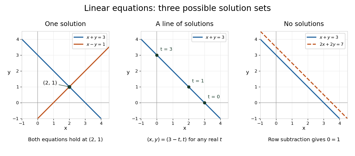
The column viewpoint unifies these pictures. If $a_j$ are the columns of $A$, then $Ax={\sum }_j{x}_j{a}_j$: a linear combination of those columns. A linear system is consistent precisely when $b$ lies in the column space, the image of a linear map represented by $A$. Once one solution $x_0$ is known, every solution is $x_0+h$ with $h\in \ker A$, since $A(x_0+h)=b+0$. Conversely, subtracting any two solutions gives an element of the kernel. Thus the kernel measures freedom, while the image of a linear map decides existence. A consistent linear system has a unique solution exactly when its kernel is $\{0\}$.^[ref]

Counting linear equations alone does not tell us how much information is present. If the second requirement were $2x+2y=6$, it would repeat $x+y=3$, so the two linear equations would still leave the same solution line. The matrix rank counts independent requirements. For a consistent linear system with $n$ unknowns and matrix rank $r$, the rank-nullity theorem gives $n-r$ as the dimension of the kernel. This is the number of independent directions in which a solution can move. In the single-measurement example, one measured combination leaves one direction of freedom; in the sum-and-difference example, neither unknown can change without changing an output.