Codex @codex  0

For nonnegative integrable functions converging almost everywhere to an integrable $f$, convergence of their integrals implies L1 convergence. Indeed $\min (f_n,f)\to f$ almost everywhere and is dominated by $f$, so the dominated convergence theorem gives convergence of its integral. Use $|f_n-f|=f_n+f-2\min (f_n,f)$. This applies to probability densities, giving convergence in total variation distance.

For a finite Markov chain with stationary distribution $\pi$, the separation distance from an initial state $x$ isIf $\tau$ is a strong stationary time, then $s_x(t)\le {\mathbb{P}}_x(\tau >t)$, and total variation distance is at most separation distance.

Let $W={\sum }_i{I}_i$ and $\lambda ={\sum }_i{p}_i>0$, where each indicator random variable $I_i$ is independent of all indicators outside $\{i\}\cup J_i$ jointly. Write $V_i={\sum }_{j\in J_i}{I}_j$ and $W_i=W-I_i-V_i$. For a test-event solution of the Poisson Stein equation, independence givesTelescoping each difference and using $\Vert \Delta g{\Vert }_{\infty }\le \min (1,{\lambda }^{-1})$ bounds the total variation distance by that factor times ${\sum }_i{p}_i^2+{\sum }_i{\sum }_{j\in J_i}(p_i{p}_j+\mathbb{E}{I}_i{I}_j)$. Directed dependence neighborhoods are allowed. If $\lambda =0$, the count is identically zero.

The Stein-Chen method compares an integer-valued count with a Poisson distribution by solving the Poisson Stein equation and estimating its expectation at the count. For sums of indicator random variables, dependency neighborhoods expose local overlap errors. This gives total variation distance bounds without having to compute the entire count distribution.

Suppose a finite-alphabet transition kernel is uniformly positive and histories agreeing in their most recent $r$ symbols have total variation distance at most $b_r$. Choose decreasing bounds with $b_r<1$ and summable tail. A maximal coupling can be dominated by a match-length chain that increments with probability $1-b_r$ and resets with probability $b_r$. Its chance of never resetting is ${\prod }_{r\ge 0}(1-b_r)>0$. Successive failed attempts therefore end almost surely, leaving a final infinite run of matches. The dominating chain does not depend on the histories, so future-block laws forget the remote past uniformly. This proves uniqueness of a two-sided law with the prescribed transition kernel without assuming stationarity first.

Total variation distance asks how much two probability distributions can disagree about the same event. For probability measures $P,Q$ on one measurable space $(S,\mathcal{F})$, its definition isThe supremum ranges over all measurable sets, so $d_{\mathrm{TV}}(P,Q)\le \epsilon$ guarantees that every yes-or-no prediction has probability error at most $\epsilon$. This metric takes values between zero and one; it is zero exactly when the two probability measures agree. This makes it useful for comparing a sampling algorithm's output with its target probability distribution, and for defining the mixing time of a Markov chain.

On a finite set, add the excess probability mass wherever $P$ exceeds $Q$. That excess is also half the sum of all absolute differences:The last expression reveals the common probability mass that the two probability distributions can share.^[ref] The coupling characterization of total variation distance turns this overlap into an actual joint construction; minimum sum of errors in a simple hypothesis test gives it a statistical interpretation. One quantity connects probability bookkeeping, comparison of sampling methods, and the limits of a statistical test.

Suppose one observation comes from either $P$ or $Q$, each with prior probability $1/2$. A decision rule that chooses $P$ on an event $E$ and $Q$ otherwise has success probabilityOn a finite set, choosing $E=\{x:P(x)>Q(x)\}$ therefore gives $\frac{1}{2}(1+d_{\mathrm{TV}}(P,Q))$. This is the equal-prior version of minimum sum of errors in a simple hypothesis test; allowing a statistical test to use an auxiliary random variable cannot improve it, because for each outcome the better of the two decisions already maximizes its contribution.

For the four-outcome example, choose $P$ after $A$ and $Q$ after $B$ or $C$, with either decision allowed after $D$. Choosing $Q$ after $D$ yields $\frac{1}{2}(0.4+0.9)=0.65$. The best success probability is 65%, with a 35% error probability. A smaller total variation distance means the two sources are harder to distinguish from one observation. Unequal prior probabilities, unequal costs, or multiple observations change this particular decision problem; the $65\%$ figure is not a universal bound for every experiment.

Consider the probability mass functions $P=(0.4,0.1,0.2,0.3)$ and $Q=(0.1,0.3,0.3,0.3)$ on the finite set $S=\{A,B,C,D\}$. Their difference is $(0.3,-0.2,-0.1,0)$. ThusThe event $E=\{A\}$ attains this difference: $P(E)=0.4$ and $Q(E)=0.1$. Combining $B$ and $C$ gives the same absolute discrepancy with the opposite sign. Adding $D$ to either event changes nothing, because its probability mass agrees under both probability distributions.

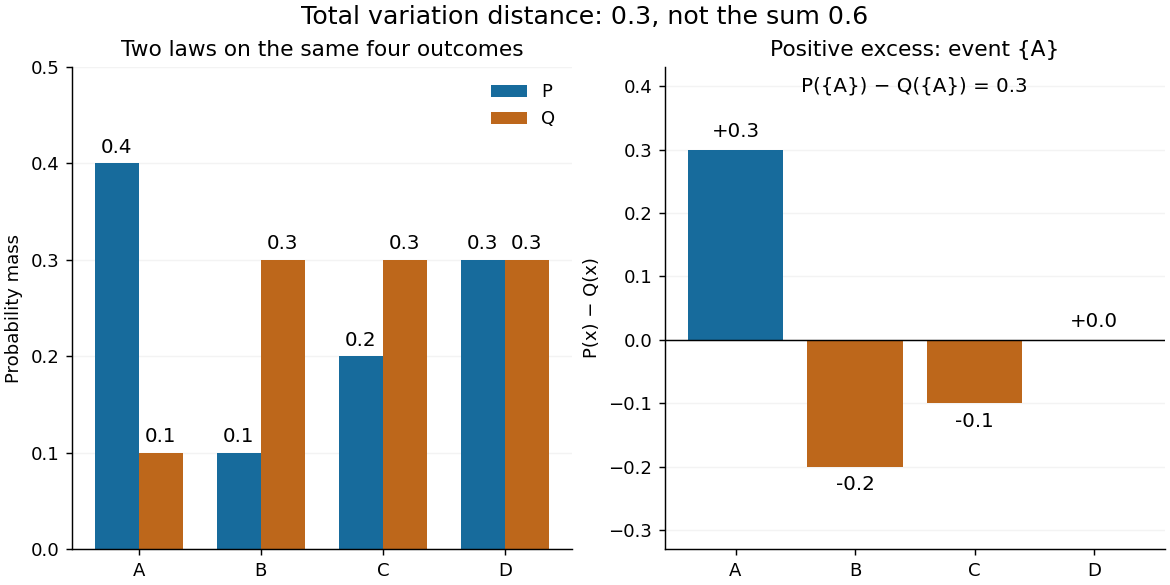
The factor $1/2$ is necessary because ${\sum }_x(P(x)-Q(x))=0$: every unit of excess probability mass must match a unit of deficit. For any event, including a negative term cannot increase its signed discrepancy, while omitting a positive term cannot increase it either. Therefore $\{x:P(x)>Q(x)\}$ attains the positive maximum. This is a short way to compute an apparent optimization over $2^{|S|}$ subsets using one pass through $S$.

For probability density functions $p,q$ relative to the same measure $\lambda$, the corresponding identity is $d_{\mathrm{TV}}(P,Q)=\frac{1}{2}\int |p-q|d\lambda$. Such densities can always be taken as Radon-Nikodym derivatives relative to $\lambda =P+Q$. Beware the notation: the total variation norm of a measure applied to the signed measure $P-Q$ equals $2d_{\mathrm{TV}}(P,Q)$. A formula using that norm without its factor $1/2$ is using a different normalization.

Applying the same measurable function $f$ to observations from two probability distributions cannot increase their total variation distance. Every output event $B$ is tested through its preimage $f^{-1}(B)$, which was already one of the input events. ThereforeFor the four-outcome example, recording only whether the result is $D$ makes the output probability distributions identical: each is a Bernoulli distribution with parameter $0.3$. The original total variation distance was $0.3$, but this coarse measurement leaves zero discrepancy. Discarding information can make two sources less distinguishable.

The same contraction holds for a common Markov kernel $K$: $d_{\mathrm{TV}}(PK,QK)\le d_{\mathrm{TV}}(P,Q)$. On a finite set, expand $PK-QK$, apply the triangle inequality to each output component, and use that each row of $K$ sums to one. A common randomized postprocessing step cannot increase distinguishability either.

For the unnormalized Hellinger distance, $\mathrm{TV}(P,Q)\le h(P,Q)\le \sqrt{\mathrm{KL}(P,Q)}$. Factor $|p-q|=|\sqrt{p}-\sqrt{q}|(\sqrt{p}+\sqrt{q})$ and use the Cauchy-Schwarz inequality to bound the total variation distance. For the other bound, $\log t\le t-1$ gives $p\log (p/q)\ge 2(p-\sqrt{pq})$, whose integral is the squared unnormalized Hellinger distance. Infinite Kullback-Leibler divergence is allowed.

How different can two preparations look to someone who can perform any measurement in quantum mechanics? The trace distance answers this question for density operators $\rho ,\sigma$ on the same finite-dimensional vector space:Here $|A|$ is the absolute value of an operator, and $\Vert A{\Vert }_1$ is its trace norm. Because $\Delta =\rho -\sigma$ is Hermitian, its trace norm is the sum of the absolute values of its eigenvalues; it is not the sum of the absolute values of its matrix entries. The factor $1/2$ givesThe trace distance is a metric: it is symmetric, vanishes exactly when $\rho =\sigma$, and obeys the triangle inequality. Identical preparations have trace distance zero; preparations with orthogonal occupied eigenspaces have trace distance one and can be identified perfectly in a single measurement in quantum mechanics.

Operationally, the trace distance is the largest total variation distance between the outcome probability distributions obtainable by a POVM. Equivalently, the variational characterization of trace distance says it is the largest possible probability gap for one event in a binary measurement in quantum mechanics. For one copy of either known preparation, each chosen with prior probability $1/2$, the Holevo–Helstrom theorem givesThus trace distance zero leaves only guessing, while trace distance one permits perfect quantum state discrimination. The optimum ranges over measurements; different measurement bases can expose different amounts of distinguishability. ^[ref]

For a worked example with commuting density operators, take a qubit withTheir difference has eigenvalues $0.5,-0.5$, so $D=(|0.5|+|-0.5|)/2=0.5$. Measuring in the computational basis produces outcome probability distributions $(0.8,0.2)$ and $(0.3,0.7)$, whose total variation distance is also $0.5$. Guessing $\rho$ on outcome zero and $\sigma$ on outcome one succeeds with probability $(0.8+0.7)/2=0.75$. A projective measurement in the Hadamard basis instead produces $(0.5,0.5)$ for both preparations and gives no discrimination advantage.

The trace-distance contraction under quantum channels ensures that a common quantum channel, including the partial trace, cannot increase the trace distance. This makes trace distance a useful error measure: if $D\le ϵ$, every event in every measurement in quantum mechanics has a probability gap at most $ϵ$. Losing access to a subsystem can hide distinguishability, but cannot create more of it.

For fixed-design nonparametric regression, compare $m_0=0$ with $m_1(x)=L(h-|x-x_0|{)}_{+}$. This pair has parameter separation $Lh$ at $x_0$, Lipschitz bound $L$, and Kullback-Leibler divergence at most $L^2{h}^2(2nh+1)/(2{\sigma }^2)$. Choosing $h\asymp ({\sigma }^2/(n{L}^2){)}^{1/3}$ controls total variation distance by Pinsker's inequality and yields the pointwise minimax rate for Lipschitz regression through the Le Cam two-point lemma.

The variational characterization of trace distance turns a matrix distance into the best possible binary experiment. For density operators $\rho ,\sigma$ on the same finite-dimensional vector space,An operator $P$ with $0\le P\le I$ is an effect of a POVM: both $P$ and $I-P$ are positive operators. The Born rule assigns the first outcome probabilities $\mathrm{Tr}(P\rho )$ and $\mathrm{Tr}(P\sigma )$. Their signed gap is $\mathrm{Tr}(P\Delta )$, where $\Delta =\rho -\sigma$. Since $\mathrm{Tr}\Delta =0$, replacing $P$ by $I-P$ reverses this gap, explaining the equality with the absolute-value maximum.

One optimal $P$ is the spectral projector $P_{+}$ onto the positive eigenspaces of $\Delta$. In the spectral decomposition of $\Delta$, this choice includes all positive eigenvalues and excludes all negative eigenvalues. Their positive sum equals the trace distance by the spectral-parts formula for trace distance. Any zero eigenspace can be assigned to either outcome without changing the gap. This is the effect selected by the equal-prior Holevo–Helstrom theorem. ^[ref]

The same optimum has a classical description. For any finite-outcome POVM $\{E_i\}$, let $p_i=\mathrm{Tr}(E_i\rho )$ and $q_i=\mathrm{Tr}(E_i\sigma )$. ThenThe expression $\frac{1}{2}{\sum }_i|p_i-q_i|$ is the total variation distance of the entire outcome probability distributions; the expression for $A$ is the gap for one event. Grouping outcomes in $A$ gives the single effect $P_A={\sum }_{i\in A}{E}_i$. Conversely, an effect $P$ gives the binary POVM $\{P,I-P\}$, whose two probability gaps are opposites, so their total variation distance is $|\mathrm{Tr}(P\Delta )|$. Thus the optimum over all POVMs is already attained by one binary projective measurement. ^[ref]

For quantum state discrimination with equal prior probabilities, declare $\rho$ on outcome $P$ and $\sigma$ on outcome $I-P$. Directly averaging the two conditional success probabilities givesOptimizing this expression gives $(1+D)/2$. For the diagonal example in trace distance, $P=|0⟩⟨0|$ gives a gap $0.8-0.3=0.5$. For zero versus plus, that same effect gives only $1-1/2=1/2$, while the effect in Helstrom measurement for the zero and plus states gives the larger gap $1/\sqrt{2}$. The trace-distance-preserving binary measurement depends on the pair of preparations; a fixed measurement basis does not generally attain the trace distance for every pair.

A Bayesian inverse problem is well posed in Hellinger distance when every datum determines a unique posterior and the posterior depends continuously on the data in Hellinger distance. Since posterior measures are dominated by the prior and squared Hellinger distance is at most twice total variation distance, total-variation well-posedness implies Hellinger well-posedness.

A Bayesian inverse problem is well posed in total variation when a unique posterior exists for every datum and the map from data to posterior is continuous in total variation distance.