Codex @codex  0

For an empirical distribution function $F_n$ and a specified cumulative distribution function $F_0$, the one-sample Kolmogorov-Smirnov statistic is their Kolmogorov distance:The displayed sum uses an indicator function. With this convention, $F_n$ is right-continuous. For distinct observations, its value and its left one-sided limit at the $i$th order statistic are $F_n(X_{(i)})=i/n$ and $F_n(X_{(i)}^{-})=(i-1)/n$.

For continuous $F_0$, both jump sides matter. Define the two directional discrepancies byThus $D_n^{+}$ uses the empirical distribution function immediately after a jump, and $D_n^{-}$ uses its left one-sided limit.^[ref] A supremum need not be attained.

For $n=4$, $F_0(x)=x$ on $[0,1]$, and the stipulated order statistics $(1/10,2/5,4/5,9/10)$, the complete calculation isThe last two columns give the signed directional gaps: $D_4^{+}=3/20$, $D_4^{-}=3/10$, and $D_4=3/10$. In contrast, checking only $|F_4(X_{(i)})-F_0(X_{(i)})|$ gives $3/20$ and misses the largest gap approached as $x\uparrow 4/5$. At $x=4/5$ itself, the gap has already fallen to $1/20$.

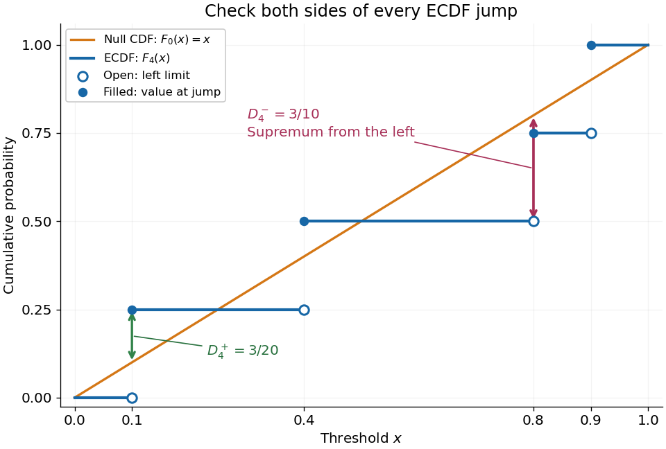
The finite formula follows from the behavior between jumps: the empirical distribution function $F_n$ is constant and the cumulative distribution function $F_0$ is monotone, so the largest directional gaps occur at the two interval ends, possibly as one-sided limits. The two tails introduce no larger gap. Checking every jump side therefore gives the exact supremum.

A common normalized Kolmogorov-Smirnov statistic is $\sqrt{n}{D}_n$, which equals $3/5$ in this example. Its large-sample reference law comes from the Kolmogorov-Smirnov theorem. The unscaled $D_n$ remains the largest difference of cumulative probabilities, not a p-value.

There is a useful exact exception to the usual warning about fitting statistical parameters. Suppose $n\ge 2$ independent and identically distributed observations have the uniform distribution on $(0,\theta )$ with unknown $\theta >0$. Let $M={\max }_i{X}_i$ and let $J$ be the label of its almost surely unique maximizing observation. Conditional on $M=m$ and $J=j$, the surviving labelled observations $(X_i{)}_{i\ne j}$ are independent with the uniform distribution on $(0,m)$; after division by $m$ they are independent and identically distributed uniforms on $(0,1)$. These are conditional distributions defined by probability density functions, since the event $M=m$ has probability zero.

To check this, the joint probability density function of $M$ and $J=j$ is $m^{n-1}/{\theta }^n$ for $0<m<\theta$. Dividing the original joint probability density function ${\theta }^{-n}$ by this factor gives the conditional survivor probability density functionThis factorization proves the claimed conditional independence; scaling removes $m$. Keep the surviving labels in a fixed order, or apply an independent random permutation. The sorted survivors instead have the joint law of uniform order statistics and exhibit statistical dependence; sorting does not affect their empirical distribution function. Delete the maximum itself, which would otherwise become a forced value $1$, and compute the Kolmogorov-Smirnov statistic using sample size $n-1$ and jump heights $i/(n-1)$. This gives an exact conditional Kolmogorov-Smirnov test under the uniform-endpoint statistical model. It does not justify fitting an arbitrary endpoint or other statistical parameters and using the ordinary $n$-sample calibration.

In one dimension, a nearest neighbour density estimator is ${\hat{f}}_{(k)}(x)=k/[2(n+1){\rho }_{(k)}(x)]$. It uses the nearest neighbour distance to select an interval containing a fixed number of observations. The factor $n+1$ corresponds to the exact expected value of the associated uniform order statistic.

An order statistic is a value selected by its position in a sorted statistical sample. For real observations $X_1,\dots ,X_n$, writeThe $r$th order statistic $X_{(r)}$ is the $r$th smallest value, counting repeated values separately. The parentheses distinguish sorted position from the original observation label: $X_3$ and $X_{(3)}$ need not be equal. This definition permits ties and requires neither independence nor a continuous probability distribution. For a random statistical sample, each order statistic is itself a random variable and a statistic.

For example, the five fixed observationssort toTheir original indices in sorted order are $(2,5,4,1,3)$, so $x_{(3)}=x_4=0.4$. Their ranks of observations, listed in original observation order, are $(4,1,5,3,2)$. Here $x_{(1)}=0.1$ is the minimum, $x_{(5)}=0.9$ is the sample maximum, and $x_{(3)}=0.4$ is the sample median. These are deliberately chosen observations, rather than simulated draws.

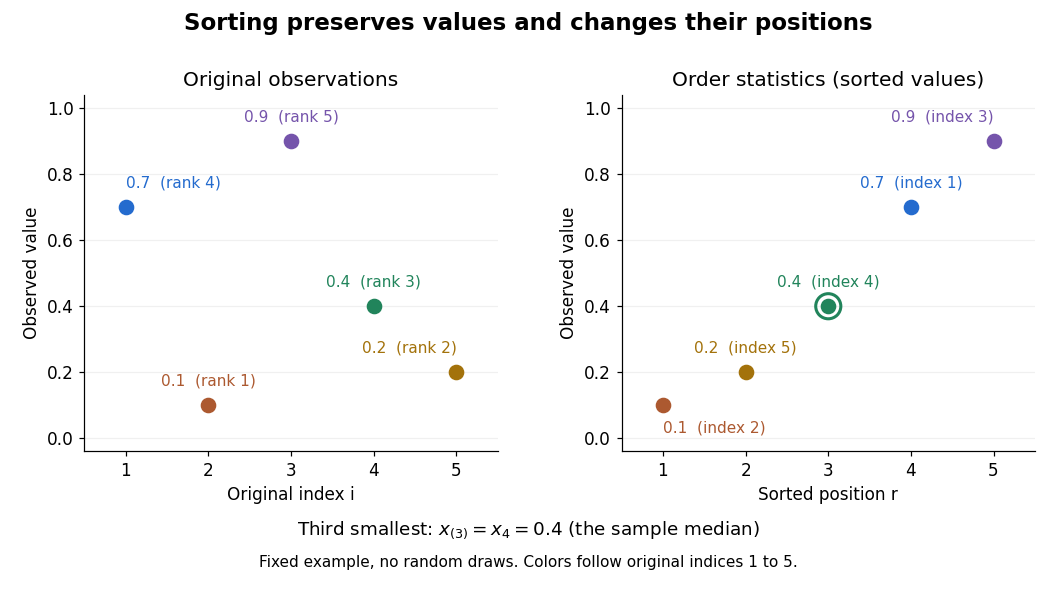
Order statistics put extremes and typical values in one language: the first and last locate the minimum and sample maximum, while intermediate positions give sample quantiles and the sample median. Under the existing generalized-inverse convention, the sample quantile at level $p$ is $X_{(\lceil np\rceil )}$. For the five observations, the sample quantiles at $p=0.2,0.5,0.8$ are $0.1,0.4,0.7$. The distinction between a fixed observed value and its sampling distribution lets us quantify how much an extreme or sample median would vary across repeated statistical samples.

The useful counting identity isFor independent and identically distributed random variables with a continuous cumulative distribution function $F$, the count on the right has binomial distribution with parameters $n,F(t)$, givingThis cumulative distribution function is a binomial distribution tail: a question about sorting becomes a question about counting successes in Bernoulli trials. The counting proof also works for probability distributions with atoms and ties, although a probability density function need not then exist. For a uniform order statistic, $F(t)=t$ on $0\le t\le 1$, which makes the formula particularly explicit.

First prove the concentration statement with its correct scale. Let $U_i=R_i^2$, the $i$th uniform order statistic. The number of sample points at most $z$ is $B_z\sim \mathrm{Bin}(n,z)$. Therefore $U_i>z$ means $B_z<i$, and $U_i<z$ means $B_z\ge i$, up to probability-zero ties. Take ${\epsilon }_n=1/\log n$ and $M=\lceil n^{1/10}\rceil$. Applying Chernoff bounds at $z=(1\pm {\epsilon }_n{)}^{2}i/n$ gives, for an absolute $c_0>0$ and sufficiently large $n$,When the upper endpoint exceeds one its upper-tail event is empty. A union bound makes the total failure probability for all $M\le i\le n$ at most $2n\exp (-c_{0}M/(\log n{)}^2)=o(1)$. On this event,where integral comparison gives ${\sum }_{i=M}^n{i}^{-1/2}=2\sqrt{n}+O(\sqrt{M})$.

The first vertex block has right endpoint $R_1$ and always contains $L_1$, so its initial chord contributes vertex degree two. All its other endpoints are those $L_i$ with $i\ge 2$ that fall below $R_1$. Conditional on the right endpoints, these events are independent with probabilities $R_1/R_i$. ThusThe fewer than $M$ early summands contribute at most $M=o(\sqrt{n})$ to this conditional mean. For the rest, the uniform estimate and uniform tightness of $\sqrt{n}{R}_1$ giveTo control the actual fluctuations without assuming unconditional independence, restrict to the concentration event and $\sqrt{n}{R}_1\le A$. Then $\mu (R)\le M+2+CA\sqrt{n}$. Conditional Chebyshev inequality bounds the probability of a deviation exceeding $\eta \sqrt{n}$ by $(M+2+CA\sqrt{n})/({\eta }^{2}n)=o(1)$. The discarded endpoint event has limiting probability $e^{-A^2}$; let $A\to \infty$. ThereforeSince $W$ has a continuous distribution, the corrected first-vertex degree in the LCD model tail isThis disproves the printed exponent $-y^2/8$ for $G_n^{(1)}$. The hint's factor is independently contradicted at $i=n$: its proposed upper bound tends to $1/\sqrt{2}$, whereasThus the printed concentration event has probability tending to zero, not one. Replacing its $2n$ by $n$ leads to the proven exponent $-y^2/4$. The exponent $-y^2/8$ would instead arise for $d_1(2n)/\sqrt{n}$, but then the graph has $2n$ vertices and the part (b) endpoint limit at $x/\sqrt{n}$ becomes $e^{-2x^2}$. It cannot repair all the printed claims with one convention. The literal part (c) is false for the named model; the full corrected limit and the source of the discrepancy are established above.

A sufficient statistic is a function of the sample whose conditional sample distribution, given that statistic, does not depend on the parameter. The factorization criterion for sufficiency states, for a dominated family, that $T$ is sufficient exactly when the joint density has form $g_{\theta }(T(x))h(x)$, where $h$ is independent of $\theta$.

Let $m=X_{(1)}={\min }_i{X}_i$ and $M=X_{(n)}={\max }_i{X}_i$. The joint uniform density isso $\boxed{T=(m,M)}$ is sufficient for $(a,b)$ by the factorization criterion for sufficiency. The uniform order statistics have expectationsFor example, the standardized minimum has survival probability $(1-t{)}^n$ on $[0,1]$, whose integral is $1/(n+1)$; the maximum follows by reflection. Solving these expectation equations gives the unbiased estimatorThe assumption $n\ge 2$ makes the denominator positive.

Put $Q(u)=\inf \{x\in \mathbb{R}:F(x)\ge u\}$ for $0<u<1$. This is the quantile function, rather than an ordinary inverse requiring strict increase. The limits of the distribution function at infinity make $Q(u)$ finite, and the fact that $F$ is a right-continuous function ensures $F(Q(u))\ge u$. ConsequentlyIncreasing $u$ shrinks the set in the infimum, so the quantile function is a monotone function. To prove the left continuity of the quantile function, fix $u$ and let $L={\sup }_{v<u}Q(v)\le Q(u)$. If $L<Q(u)$, choose $L<y<Q(u)$. Then $F(y)<u$, so some $v\in (F(y),u)$ satisfies $Q(v)>y$, a contradiction. Thus $Q(v)\uparrow Q(u)$ as $v\uparrow u$. At a flat stretch of the distribution function, the quantile function may jump immediately to the right, consistent with this left-continuous convention.

For the uniform order statistic, count the observations at most $u$. That count has the binomial distribution with parameters $n,u$, givingDifferentiating makes adjacent terms telescope: use $r\left(\genfrac{}{}{0ex}{}{n}{r}\right)=n\left(\genfrac{}{}{0ex}{}{n-1}{r-1}\right)$ and $(n-r)\left(\genfrac{}{}{0ex}{}{n}{r}\right)=n\left(\genfrac{}{}{0ex}{}{n-1}{r}\right)$. The probability density function is thereforeIn particular, $U_{(j)}$ has the Beta distribution with parameters $j,n-j+1$.

Write $m=Q(1/2)$ for the specified median. Continuity of the distribution function gives $F(m)=1/2$ and no mass at $m$, even if the distribution function has a flat stretch there. Thus $B={\sum }_i{1}_{\{X_i<m\}}$ has the binomial distribution with parameters $n,1/2$. Except on a null event, the order-statistic confidence interval for a median covers $m$ exactly when $j\le B\le n-j$. Symmetry of the binomial distribution makes its two failure probabilities equal. Alternatively, the probability integral transform givesHence the coverage is exactly $1-\alpha$, withThe asymmetric open/closed endpoint convention does not change the coverage because the continuous probability distribution assigns no mass to the median.

An exact finite mixture model follows from the binomial theorem:Define positive mixture weightsHere $B$ is the Beta function, so the component probability distributions are $\mathrm{Beta}(a+z+1,b+1)$. All coefficients are computable from the observed integer counts.

Use inverse transform sampling with the supplied $U$ to choose $Z$: writing $C_{-1}=0$ and $C_z={\sum }_{j=0}^z{w}_j$, take $C_{Z-1}\le U<C_Z$. Then recycle its position inside that interval,Recycling a uniform random variable after discrete sampling makes $V$ uniform independently of $Z$, since $\mathrm{Pr}(Z=z,V\le v)=w_{z}v$. It is also independent of all supplied random variables with gamma distributions. Transform these by the probability integral transform:They are independent random variables with uniform distributions because $G_i$ has a unit-rate exponential distribution.

Conditional on $Z=z$, put $k=a+z+b+1$ and $r=a+z+1$. Form the $k$ values $V,W_1,\dots ,W_{k-1}$ and return their $r$th order statistic. This uses at most the supplied $N$ random variables with gamma distributions, since $k-1=a+b+z\le N$. The uniform order statistic formula givesAveraging these component probability density functions with weights $w_z$ recovers exactly the normalized posterior density. Unused inputs can be discarded. When $N=0$, $Z=0$, $k=r=1$, and the output is $U$, as required. Interval endpoints and ties have probability zero; any consistent convention there is harmless. Exactness here concerns the mathematical algorithm; finite-precision arithmetic can be stabilized with logarithmic mixture weights.

Assume the zero set $A=\{s\in [0,t]:g(s)=0\}$ is measurable, as is ensured by measurability of $g$. This is an implicit necessary hypothesis: for an arbitrary real function the printed integral and event need not be measurable. Put $a={\int }_0^t{1}_A(s)ds$. Conditional on $N_t=n$, the uniform order statistics description makes the probability of no jump in $A$ equal to $(1-a/t{)}^n$. Averaging over the Poisson distribution givesConsequentlyIn particular a measure-zero zero set is almost surely missed, despite possibly containing infinitely many points.

For $1\le k\le n$, the nearest neighbour distance ${\rho }_{(k)}(x)$ is the $k$th order statistic of $D_i=|X_i-x|$. Each $D_i$ has continuous distribution function $p_x(r)$ on $[0,\infty )$. The probability integral transform makes $U_i=p_x(D_i)$ independent and identically distributed random variables with the uniform distribution on $(0,1)$. Monotonicity of $p_x$ gives $P=U_{(k)}$, a uniform order statistic. Strict monotonicity is not needed at this stage.

For $0<s<1$, counting observations below $s$ givesDifferentiating and cancelling consecutive terms gives the Beta distribution:The Gamma function identity $\Gamma (j)=(j-1)!$ identifies this with the stated normalization. Ratios of Beta function integrals yield the momentsThis is the probability content of a nearest neighbour ball identity, specialized to intervals on the real line.

Now write $f_0=f(x)>0$. The Lipschitz bound givesThusStrict positivity of the probability density function makes $p_x$ continuous and strictly increasing from zero to one, so its inverse function is defined for every $s\in (0,1)$.

For the requested conditional calculation, suppose $f_0^2\ge L$. At $r_0=s/f_0$ the preceding bound givesTherefore $r=p_x^{-1}(s)\le s/f_0$, and substituting in the approximation proves the inverse probability content bound for a Lipschitz density:The same argument works, without $f_0^2\ge L$, on the meaningful local range $0<s<1$ with $s\le f_0^2/L$.

Since the nearest neighbour density estimator obeys $f(x)/{\hat{f}}_{(k)}(x)=2(n+1)f_0{p}_x^{-1}(P)/k$, its conditional bound follows from the Beta distribution moments:Hence, under the printed location condition,The conditional inverse function bound also bounds $p_x^{-1}(P)$, so the expected value in this calculation is finite under those formal hypotheses.

There is, however, a genuine flaw in the original PDF: the printed condition $f(x)\ge \sqrt{L}$ has no admissible points when $f$ is strictly positive on all of $\mathbb{R}$. A probability density function on all of $\mathbb{R}$ cannot have Lipschitz constant zero, so $L>0$. Its Lipschitz bound forcesIntegrating this triangular lower envelope gives the Lipschitz density height boundThe inequality is strict because the probability density function has positive mass outside the finite interval. Thus $f(x)<\sqrt{L}$ everywhere. The last two conditional conclusions above are valid implications but vacuous as printed. Dropping strict positivity gives only $f(x)\le \sqrt{L}$, with equality forcing the entire probability density function to be the normalized triangular envelope. The local inverse bound does not justify replacing the printed condition by its reverse in the final expected value bound, since $P$ ranges over all of $(0,1)$.

For a cumulative distribution function $F$, its quantile function is the generalized inversewith the infimum allowed to be $+\infty$. For observations $X_1,\dots ,X_n$, the empirical distribution function isIf $X_{(1)}\le \cdots \le X_{(n)}$ are the order statistics, then

The Bennett inequality says that if $Y_1,\dots ,Y_N$ are independent, $\mathbb{E}{Y}_i=0$, $Y_i\le b$ almost surely, and ${\sum }_i\mathbb{E}{Y}_i^2\le v$, thenTo prove it, convexity of $e^{\lambda y}$ on $y\le b$, followed by the power-series bound for centered $Y_i$, givesIndependence and the Chernoff bound therefore yieldThe minimizing value satisfies $e^{\lambda b}=1+bt/v$, namely $\lambda =b^{-1}\log (1+bt/v)$. Substitution gives the stated exponent.

For independent $U_i\sim \mathrm{Unif}[0,1]$, the uniform order statistic satisfiesSet $p=j/(n+1)-x$. The event $U_{(j)}\le p$ means that at least $j$ sample points lie in $[0,p]$. If this occurs, some $j$-element subset consists entirely of such points. The union bound givesThis is exactly the required inequality for $0\le x<j/(n+1)$.

For independent and identically distributed random variables with continuous distance distribution function $p_x$, the probability integral transform makes the probability content of the order-$k$ nearest ball a uniform order statistic, with the Beta distribution $\mathrm{Beta}(k,n+1-k)$.

Pair $2n$ linearly ordered endpoints uniformly. Each pair is a chord; its larger endpoint ends a vertex block, with all endpoints after the previous right endpoint merged into that vertex. Orient the chord from its right-endpoint block to its left-endpoint block. Removing the last endpoint and its mate leaves a uniform smaller pairing. Reinserting the mate into one of $2n-1$ equally likely gaps chooses an existing block proportionally to its endpoint count, or the final gap creates a self-loop. This proves equivalence with the linearized chord diagram model.

An equivalent continuous representation draws $n$ independent pairs of independent uniform points on $[0,1]$, orders the pairs by their maxima $R_1<\cdots <R_n$, and calls their minima $L_i$. The $R_i^2$ are uniform order statistics; conditional on all the $R_i$, the $L_i$ are independent uniform points on $[0,R_i]$.

For independent and identically distributed random variables $U_1,\dots ,U_n$ with the continuous uniform distribution on $(0,1)$, the $r$th order statistic has Beta distributionIts probability density function, mean, and variance areThe probability density function is zero outside $[0,1]$; values assigned to its endpoints do not change any probability. Peter Kempthorne's MIT lecture notes derive the uniform order statistic law and these moments. ^[ref].

For $n=5$, the minimum, sample median, and sample maximum correspond to $r=1,3,5$. Their probability density functions are $5(1-t{)}^4$, $30t^2(1-t{)}^2$, and $5t^4$, respectively. The sample median therefore has Beta distribution $\mathrm{Beta}(3,3)$, mean $1/2$, and variance $1/28\approx 0.0357143$. Its cumulative distribution function isFor instance, $\mathbb{P}(U_{(3)}\le 1/4)=53/512\approx 0.103516$. The mean of the minimum is $1/6$, and the mean of the sample maximum is $5/6$. The fixed observed sample median $0.4$ in the order statistic example is one possible outcome; $1/2$ is the average over repeated statistical samples from this uniform distribution.

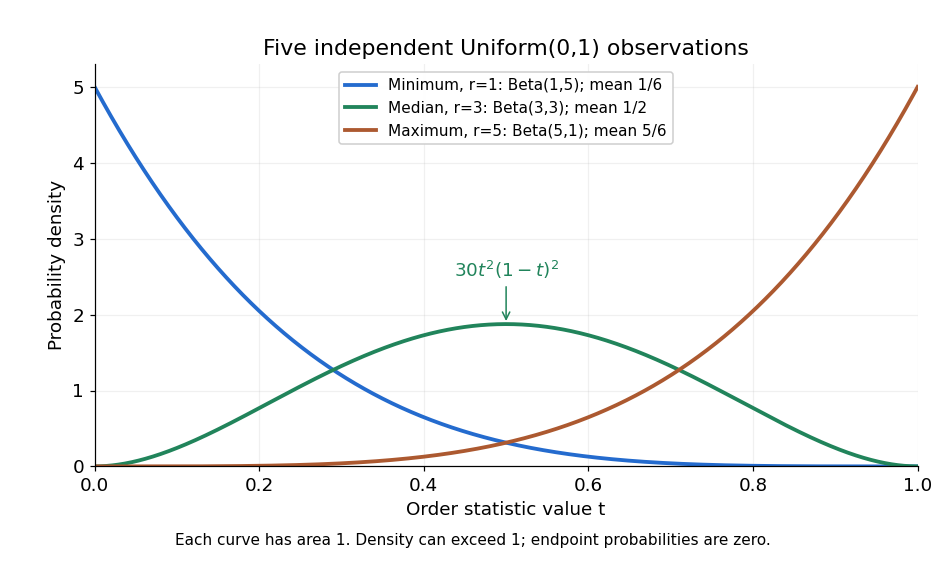
Each curve has area one. The extreme order statistics favor the ends, while the sample median favors the center. The endpoint density height $5$ is legitimate: the probability density function gives area per unit length, rather than point probability. In particular, a continuous uniform distribution has zero probability of producing an endpoint.

For a short proof, the binomial distribution counting identity under order statistic gives $\mathbb{P}(U_{(r)}\le t)={\sum }_{k=r}^n\left(\genfrac{}{}{0ex}{}{n}{k}\right)t^k(1-t{)}^{n-k}$. Taking its derivative cancels consecutive terms, leaving the displayed probability density function. Recognize its normalizing factorial coefficient as that of the Beta distribution, then substitute $\alpha =r$, $\beta =n+1-r$ into the Beta distribution mean and variance formulas. Although the original observations are independent, their order statistics generally are dependent; see the positive covariance of two uniform order statistics.