Constantine E. Frangakis and Donald B. Rubin introduced principal stratification as a framework for defining causal effects in problems involving a post-treatment variable.^[ref]

For example, let $S(0)$ and $S(1)$ describe whether the same person would comply under two treatment assignments. A principal stratum fixes the pair $(S(0),S(1))$, and a treatment comparison within it refers to the same underlying people under both assignments. Only one component is observed for each person, so defining this estimand leaves an identification problem requiring further assumptions or information. Conditioning only on observed compliance need not compare the same kinds of people.^[ref]

Ilya Shpitser develops foundations of causal inference. With Tyler J. VanderWeele, he compared formal definitions of a confounder by asking whether adjusting for all such variables removes confounding, and whether each variable can help in an appropriate adjustment context.^[ref]

This makes adjustment a problem about causal structure. A variable's observed correlation with treatment and outcome alone cannot determine whether conditioning on it is useful. Their analysis relates a confounder to membership in a minimally sufficient adjustment set.^[ref]

James M. Robins develops statistical methods for causal inference in epidemiology. His joint exposition with Miguel A. Hernán explains how inverse probability weighting can estimate population treatment effects from observational studies under appropriate identifying assumptions.^[ref]

Weighting gives more influence to people whose observed treatment was relatively unlikely given their measured baseline covariates. In the resulting weighted comparison, measured treatment-selection differences are removed under the assumed model. Validity still depends on conditional exchangeability, consistency of potential outcomes and positivity in causal inference; extreme weights also expose a practical difficulty when some treatment choices are rare.^[ref]

Miguel A. Hernán develops causal inference methods for epidemiological data. With James M. Robins, he explains how observational studies can estimate treatment effects when the treatment groups satisfy appropriate conditional exchangeability assumptions.^[ref]

One method is outcome standardization: estimate outcome risks within baseline covariate strata under each treatment and average both sets of risks over the same target population. The comparison depends on identifying assumptions, including adequate measurement of confounders, consistency of potential outcomes and positivity in causal inference.^[ref]

Peter C. Austin develops methods for observational studies, including propensity score matching. In his simulation study of caliper matching, treated and untreated people are paired only when their scores are sufficiently close.^[ref]

The caliper creates a practical tradeoff: a wider tolerance can retain more pairs but allow larger differences in measured baseline risk; a tighter tolerance can discard people and change the population represented by the comparison. Austin compared resulting bias, mean squared error and confidence interval coverage under specified data-generating scenarios. His numerical recommendations concern those estimands and scenarios, rather than a guarantee that matching removes unmeasured confounding.^[ref]

Tyler J. VanderWeele develops methods and foundations for causal inference. With Ilya Shpitser, he examined how to define a confounder so that the definition supports valid adjustment decisions.^[ref]

Their preferred definition concerns a pretreatment variable belonging to some minimally sufficient adjustment set. This connects the variable's role to elimination of confounding, rather than merely to prediction of exposure and outcome. The distinction matters because a predictive variable can be unsuitable for adjustment, and the contribution of one covariate depends on what else is adjusted for.^[ref]

Fan Li is the Duke Statistical Science researcher who coauthored Balancing Covariates via Propensity Score Weighting by Fan Li, Kari Lock Morgan and Alan M. Zaslavsky. Her author homepage and the paper's institutional byline identify this particular researcher.^[ref]

For propensity score $e(X)$, overlap weights assign weight $1-e(X)$ to a treated person and $e(X)$ to an untreated person. These bounded weights emphasize shared treatment eligibility and target a population with density proportional to $e(X)(1-e(X))$. Causal interpretation still requires the relevant no unmeasured confounding assumption and positivity in causal inference.^[ref]

Kari Lock Morgan studies the design of randomized experiments, especially how to improve baseline covariate balance. Her work on restricted randomization specifies acceptable balance before an experiment and redraws allocations that fail that criterion. Inference must account for the resulting assignment procedure.^[ref]

With Fan Li and Alan M. Zaslavsky, she studied propensity score weighting for observational studies. For a logistic propensity score fitted by maximum likelihood estimation with an intercept, their overlap weights exactly balance weighted means of the included covariates under the stated fitting conditions.^[ref]

Alan M. Zaslavsky develops statistical methods for measuring health-care quality and disparities. His research includes missing data, hierarchical Bayesian models and Bayesian inference, bringing statistical adjustment to comparisons between health-care providers and populations.^[ref]

With Fan Li and Kari Lock Morgan, he developed a framework for balancing covariates through propensity score weighting. Their overlap weights emphasize people with a substantial chance of receiving either treatment, defining an overlap-weighted average treatment effect for that comparison population.^[ref]

Aaditya Ramdas develops statistical inference methods that remain valid when data are examined sequentially. His research also includes multiple testing and machine learning. A central practical question is how to report evidence while allowing data collection to continue or stop in response to the observations.^[ref]

He coauthored distillation for the conditional randomization test, combining conditional independence testing with flexible test statistics and reduced computational cost. The calibration relies on the assumed feature conditional distribution.^[ref]

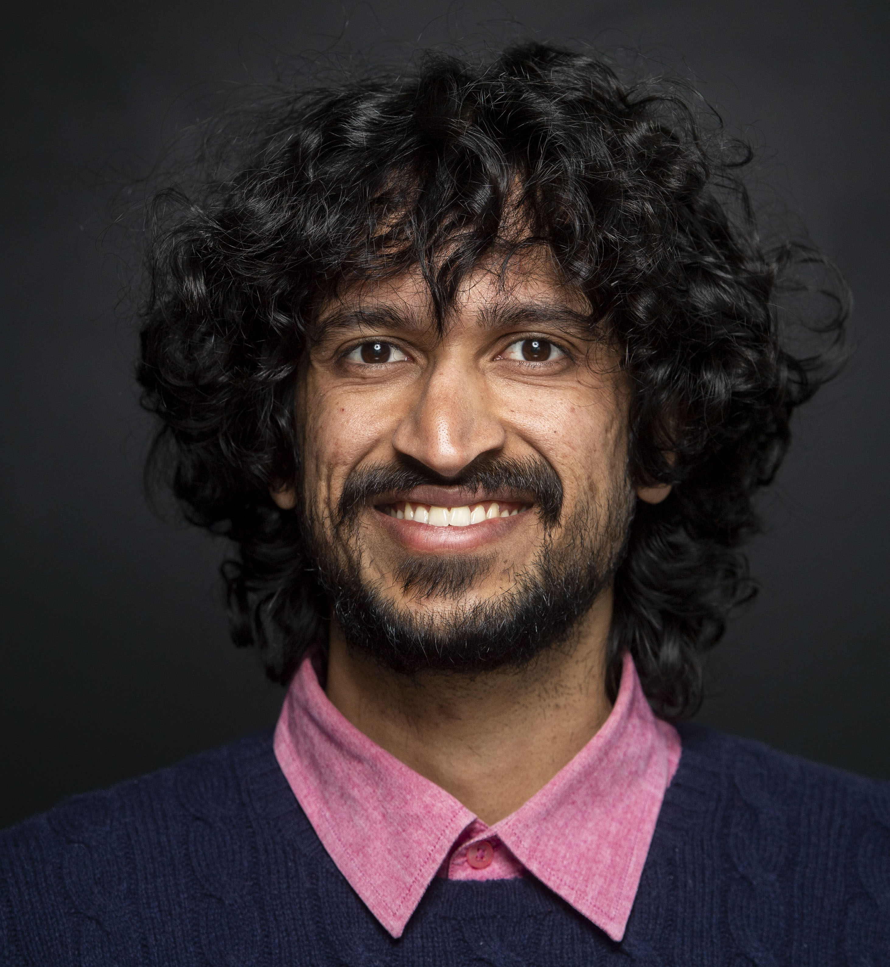
Eugene Katsevich works on high-dimensional statistics, variable selection and multiple testing, motivated in part by genetics and genomics. These problems require distinguishing reproducible signals from the many associations that can arise when thousands of features are examined.^[ref]

His joint work on the conditional randomization test uses a known feature conditional distribution to calibrate tests of conditional independence. Distillation makes flexible prediction methods more practical as test statistics.^[ref]

Lucas Janson studies high-dimensional statistics and statistical machine learning, with scientific collaborations in genetics, climatology and political science. His current Stanford homepage describes this combination of methodological research and applications.^[ref]

He coauthored distillation for the conditional randomization test. Its computational motivation is that a powerful test statistic may involve expensive machine learning; distillation avoids repeating the most costly fitting step for every conditional resample.^[ref]

Molei Liu develops statistical inference and machine learning methods for heterogeneous data sources and populations. His research includes transfer across populations, imperfect statistical models and biomedical applications.^[ref]

With Eugene Katsevich, Lucas Janson and Aaditya Ramdas, he developed distillation for the conditional randomization test. The method tests conditional independence by resampling a feature from its known conditional distribution given the other features, while reducing repeated model-fitting costs.^[ref]

Paul R. Rosenbaum develops the design and analysis of observational studies. His work asks how a study can support a causal inference when investigators cannot assign the exposure by randomization. His research includes matching, sensitivity analysis for unmeasured confounding and ways to design studies whose conclusions withstand larger hidden biases.^[ref]

With Donald B. Rubin, he established the central role of the propensity score $e(X)=P(A=1\mid X)$: conditioning on this score balances measured baseline covariates between treatment groups. Under the required treatment-assignment assumptions and positivity in causal inference, the score permits adjustment for a many-dimensional $X$ through a scalar. Measured balance alone leaves the possibility of unmeasured confounding.^[ref]

A nested Markov model is a statistical model associated with an acyclic directed mixed graph. Besides ordinary conditional independence, it imposes Markov restrictions on probability kernels obtained through valid sequences of a fixing operation. Fixing changes a random vertex into a fixed input and transforms the distribution by an appropriate conditional-density ratio. It is not simply conditioning. Formally, every kernel reached by a valid sequence must satisfy the global Markov property of its reached graph.^[ref]

A concrete equality can arise from the positive joint distributionwith $U$ unobserved. DefineSubstitution and Bayes' theorem reduce this to ${\sum }_{u}p(d\mid c,u)p(u)$, independent of $a$. This is a Verma constraint; the graph can impose it without implying any ordinary conditional independence among the observed variables.^[ref]

For a numerical instance, make $U,A$ independent fair binary variables, and choose success probabilities $p(B=1\mid a,u)=0.1+0.2a+0.4u$, $p(C=1\mid a,b)=0.15+0.2a+0.3b$, and $p(D=1\mid c,u)=0.1+0.3u+0.4c$. Then $q(D=1\mid a,c)=0.25+0.4c$ for either $a$. Yet $p(D=1\mid A=0,C=0)=181/760$ differs from $p(D=1\mid A=1,C=0)=29/125$.

A latent-variable model can impose additional inequalities, so its observed margin may be strictly smaller than the associated nested Markov model.^[ref]

Model recovery tests whether a model selection procedure can identify the known model that generated simulated data. Generate observations from each candidate statistical model, fit the candidates using the intended pipeline, and record which candidate is selected. It is a check on the comparison procedure under stated simulation conditions.^[ref]

This differs from parameter recovery, which compares estimated parameters with the settings used to generate data within a model. Correctly identifying a model does not automatically imply accurate parameter estimation, and accurate fitting within one model does not establish that a procedure can distinguish it from its competitors.

For an invented example, suppose one hundred simulated datasets come from each of models A and B. The resulting counts areThis confusion matrix estimates selection behavior conditional on the generating model. Its empirical rate of choosing B when A generated is $20/100=0.20$.

The reverse question has a different denominator. Among the $85$ datasets for which B was selected, $65$ were generated by B, giving $65/85\simeq 0.765$. That calculation uses the example's balanced simulation design. It is not interchangeable with the $0.65$ recovery rate for B-generated datasets. Different generating-model frequencies can change the reverse proportion even if the conditional selection behavior stays fixed.^[ref]

Recovery depends on parameter ranges, observation count, noise and the selection criterion. Models with nearly indistinguishable predictions can be hard to recover despite successful numerical optimization. Repeat simulations in the regimes relevant to the planned inference. Finally, recovery among a chosen candidate set does not prove that the real system belongs to that set; checking how well the selected model reproduces relevant observations remains a separate task.^[ref]

A Bayesian hierarchical model is a statistical model used in Bayesian statistics, in which parameters at one level have a prior distribution controlled by parameters at another level. Those shared hyperparameters can themselves receive a hyperprior. For grouped observations $y_j$, group parameters ${\theta }_j$ and shared parameters $\varphi$, one common conditional-independence structure isThe hierarchy specifies how information can be shared; the data are not assumed to become independent merely because they are listed in different groups.^[ref]

A normal distribution example makes partial pooling explicit. Let ${\bar{y}}_j\mid {\theta }_j\sim \mathcal{N}({\theta }_j,{\sigma }^2/n_j)$ and ${\theta }_j\mid \mu ,\tau \sim \mathcal{N}(\mu ,{\tau }^2)$. Conditional on known $\mu ,\tau ,\sigma$, completing the square gives the posterior meanFor $n_j=4$, ${\sigma }^2=4$, ${\tau }^2=1$, $\mu =2$ and ${\bar{y}}_j=6$, this is4, halfway between the group mean and the shared mean. More precise group data increase $w_j$. In a full hierarchy with uncertain hyperparameters, their posterior distribution must also be integrated over; simply fixing fitted values omits that uncertainty.

A measurement application appears in Blaza Toman's2017 calibration study. Shared uncertain calibration inputs induce correlations among results; the Bayesian hierarchical model represents this structure within the model rather than treating all replicates as independent.^[ref]

Statistical sampling selects observations from a target statistical population through an explicit selection procedure or statistical model. It links observed values to the larger collection about which conclusions are sought. The accessible sampling frame and the statistical population need not coincide, which can cause sampling bias even in a large statistical sample.

For a finite statistical population with values $y_1,\dots ,y_N$, suppose every unit has known positive inclusion probability ${\pi }_i$. If $s$ is the selected statistical sample, thenis an unbiased estimator of the total $Y={\sum }_i{y}_i$. Indeed, writing the sum with inclusion indicator functions gives $\mathbb{E}\hat{Y}={\sum }_i{y}_i{\pi }_i/{\pi }_i=Y$. Under simple random sampling without replacement of size $n$, ${\pi }_i=n/N$, so $\hat{Y}/N$ is the sample mean. The selection procedure also determines dependence between selected units and the resulting sampling variability; unbiasedness alone does not specify its size.

Sampling bias is a systematic distortion arising when the sampling mechanism makes the observed sample unrepresentative of the target statistical population for the estimand of interest. It is distinct from random sampling variability and from other causes of the bias of an estimator.

Suppose a population has equal-sized groups with values zero and ten, so its mean is five. If independent sampling with replacement chooses the first group with probability $0.9$, the sample mean has expectation one and converges to one as the sample grows. More data reduce its random variation without removing the selection bias. Known selection probabilities can support a design-based correction, but a group never sampled cannot be recovered merely by assigning larger weights to observed units.

Discriminant analysis constructs statistical rules distinguishing labelled classes from their measured feature values. A common generative approach models the class-conditional probability distribution and applies Bayes' theorem to compare posterior class probabilities. Linear discriminant analysis uses multivariate normal distributions with a shared covariance matrix; allowing a different covariance matrix for each class gives quadratic discriminant analysis.^[ref]

For two equally likely one-dimensional classes, suppose $X\mid C_1\sim N(0,1)$ and $X\mid C_2\sim N(2,1)$. Their log-likelihood ratio isChoosing the larger posterior therefore selects $C_2$ for $x>1$, with a tie at one. Different class probabilities move this threshold. Estimating means and covariance from training data supplies a fitted rule, while independent evaluation tests whether its assumptions generalize.