A confidence score is a numerical output used to express how strongly a system supports a prediction, particularly in statistical classification. Its meaning depends on the system: it may be an estimated probability, a distance from a decision boundary, or another score whose ordering is useful. A number between zero and one does not by itself establish a probability interpretation. Probability calibration concerns whether predicted probabilities agree with observed frequencies.^[ref]

Consider a synthetic binary statistical classification example. Among $100$ independent test cases assigned a positive-class score near $0.8$, suppose $80$ actually belong to that class. Their observed fraction $80/100=0.8$ agrees with the average predicted probability. If only $60$ belong to the positive class, the same scores overstate the observed positive frequency in this group. A reliability diagram groups predictions by their estimated probability and compares each group's mean prediction with its observed positive fraction. Finite groups have sampling variation, so agreement in one group is evidence to assess with its sample size, rather than a guarantee about each case.^[ref]

Ordering and probability calibration answer different questions. For scores $s$ in $[0,1]$, replacing every score by $s^3$ preserves their order but changes $0.8$ to $0.512$. Thus an unchanged ranking can accompany very different probability statements. Conversely, a system assigning the overall positive fraction to every case can have useful aggregate probability calibration while failing to distinguish cases.

A confidence score can support a threshold for accepting a prediction or passing it to another process. Select and assess that threshold using examples separate from model fitting and representative of the intended inputs. A threshold does not establish its own error rate; observations on suitable test data supply that evidence. Distinguish a positive-class probability from the score of whichever class was selected: they are different quantities when the selected class changes.

Probability calibration means that reported probabilities agree with the frequencies of the outcomes they describe. For binary classification, let $Y\in \{0,1\}$ be the true label and let $P\in [0,1]$ be the predicted positive-class probability. Population calibration is the conditional expectation conditionAmong cases receiving a value near $0.8$, the positive fraction should therefore be near $0.8$, with uncertainty in any finite sample.^[ref]

A simple example separates calibration from discrimination. Suppose the population has a positive fraction of $0.3$ and a predictor always reports $P=0.3$. Then $\mathbb{E}[Y\mid P]=\mathbb{E}[Y]=0.3$, so it is calibrated, although it cannot rank one case above another. Conversely, replacing a useful score $s$ by a strictly increasing transformation such as $s^3$ preserves ranking but generally changes the claimed probability. Thus ordering cases and attaching reliable numerical probabilities are different tasks.

A reliability diagram estimates the agreement by grouping predictions and comparing each group's mean prediction with its observed outcomes. Assess it using suitable held-out observations. A calibrator fitted to predictions on the same observations used to fit the original model can inherit an overly optimistic picture of performance; fitting and evaluation need appropriate separation.^[ref]

A 2017 study found substantial confidence miscalibration in the evaluated neural networks, even when prediction accuracy improved. It also tested temperature scaling as a compact post-processing adjustment. These were empirical results on specified models and datasets, rather than a theorem that all neural networks are miscalibrated.^[ref]

Within-observer agreement versus reference agreement distinguishes consistency of an observer's repeated labels from concordance with a separately defined reference. The first asks whether the observer repeats a decision; the second asks whether that decision matches the comparison standard. In statistical classification, neither quantity can replace the other.

For $n$ cases, let $X_{i1}$ and $X_{i2}$ be one observer's labels at two readings, and $Y_i$ the reference label. Define the two empirical agreement fractionsAn original binary example has 100 cases, half reference-positive and half reference-negative. An observer reverses every reference label and repeats that reversal on the second reading. Then $A_{\mathrm{within}}=1$ while $A_{\mathrm{ref}}=0$. Perfect repeat agreement can coexist with complete reference disagreement. An observer always assigning the negative label also has perfect repeat agreement, but only 50 percent reference agreement in this balanced example.

A confusion matrix shows which categories contribute to disagreement, whereas a single overall percentage can conceal systematic shifts or an imbalanced case mix. Reference agreement is classification accuracy relative to that reference, not proof that the reference is infallible. A consensus panel, a later outcome and an independent molecular test answer different validation questions.

A primary 2017 study made this distinction experimentally by having pathologists interpret skin-biopsy sets twice, at least eight months apart, and comparing their interpretations with an experienced consensus reference. The study started with 240 cases and reported reproducibility separately from reference concordance.^[ref] The delayed repeat reduced immediate recall, but did not transform repeated judgments into independent biological truths.

A useful evaluation preserves case identity, reading order and the exact reference procedure. If a machine learning classifier learns an observer's systematically shifted labels, it may reproduce that observer well while disagreeing with the external reference. Reporting both comparisons makes that limitation visible. Uncertainty estimates should also account for repeated cases and multiple readings rather than counting every label as an independent subject.

Static equilibrium is a state in which a mechanical system remains at rest in a specified reference frame. For a rigid body in an inertial frame, zero resultant external force and zero resultant external torque are the balance conditions:The body must also initially be at rest: zero acceleration alone does not exclude uniform translation or steady rotation.^[ref]

A free-body diagram identifies the body being analyzed and includes its external loads and support reactions. Internal action–reaction pairs cancel when both interacting parts belong to the chosen system. Choosing a different point $O$ for the torques changes their sum by a term proportional to the resultant force. Thus, when the resultant force is zero, a vanishing resultant torque about one point also vanishes about any other point.^[ref]

For an original example, take an ideal massless horizontal beam of length $4\mathrm{m}$, supported at its ends, with a downward $120\mathrm{N}$ load $1\mathrm{m}$ from the left support. Let the upward support reactions be $R_L$ and $R_R$. Vertical force balance and torque balance about the left end giveso $R_R=30\mathrm{N}$ and $R_L=90\mathrm{N}$. The nearer support carries more load because the farther reaction has the larger moment arm. Two equal and opposite forces alone would not guarantee equilibrium: a force couple can have zero resultant force and a nonzero torque.

A simple apparatus test suspends a beam from two spring balances and moves a known load along it. Account separately for the beam's own gravitational weight and its center of mass before comparing the measured reactions with the ideal calculation. The sum of the readings should track total downward load, while their difference changes with load position. Finally, static equilibrium does not imply dynamical stability: an exactly upright inverted pendulum balances at rest but departs from that state after a small disturbance.

A support polygon is the convex hull of a body's supporting contact positions, projected onto a horizontal plane. For a rigid body resting on that plane in a uniform gravitational field, with gravity as the only applied load besides support reactions, it describes which horizontal center of mass positions can admit static equilibrium. Widely separated feet can support a center of mass above empty space between them: the footprint's convex hull, rather than the material under every point, matters.^[ref]

The geometry follows directly from force and torque balance. Let the contact positions be $(x_i,y_i,0)$ and their upward normal forces be $N_i\ge 0$. The inequality expresses unilateral contact: an ordinary unbonded support can push the body upward but cannot pull it downward. For total mass $m>0$, gravitational acceleration $g>0$ and horizontal center of mass projection $c=(x_c,y_c)$, balance givesDivide by $mg$ and write ${\lambda }_i=N_i/(mg)$. ThenThus $c$ must be a convex combination of the contacts, which is exactly membership in their convex hull. Conversely, any such convex combination supplies nonnegative reactions $N_i=mg{\lambda }_i$ satisfying this model's balance equations. The center of pressure of these vertical contact forces coincides with $c$. This proves existence of allowable reactions; it does not determine every reaction uniquely when there are more contacts than independent balance equations.

For an original three-foot example, take contact positions $(0,0)$, $(1,0)$ and $(0,1)$ in metres. The support polygon is the triangle described by $x\ge 0$, $y\ge 0$, $x+y\le 1$. A $10\mathrm{kg}$ body with $c=(0.30,0.20)\mathrm{m}$ requires the convex combination coefficientsWith $g=9.81m/{\mathrm{s}}^2$, the corresponding normal forces are $49.05$, $29.43$ and $19.62\mathrm{N}$. Moving the projection to $(0.70,0.50)\mathrm{m}$ would require ${\lambda }_1=-0.20$, a downward reaction at the first foot. No set of nonnegative normal forces can hold that configuration at rest under the stated loads.

A simple test uses a rigid plate on three small supports, a movable known mass, and three load cells measuring the upward reactions. Include the plate's own mass and center of mass when calculating the combined projection. As that projection approaches the edge $x+y=1$, the first support's reading approaches zero. Beyond the edge, maintaining the same contact configuration would require the forbidden downward reaction; the observed motion or changed contact set marks the failure of the original static equilibrium. This is a proposed apparatus test of the balance equations, not reported experimental data.

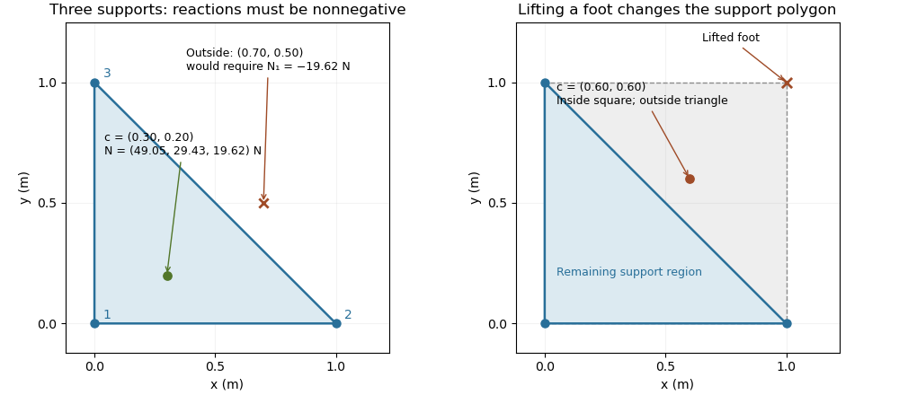
The distance from an interior projection to the polygon's nearest edge is a static tipping margin; here it is $\min (0.30,0.20,0.50/\sqrt{2})=0.20\mathrm{m}$. A boundary projection has zero margin: some supports unload, and an arbitrarily small outward shift can make balance impossible. A strictly interior projection gives a positive geometric margin against small horizontal shifts under the same model. It is not a general certificate of dynamical stability for a flexible or articulated system.

This explains a constraint in a quadrupedal robot's gait. Four feet at the corners of a square give a square support polygon. Lifting the corner $(1,1)$ leaves the triangle $x\ge 0$, $y\ge 0$, $x+y\le 1$. A center of mass projection at $(0.60,0.60)$ was inside the square but is outside that triangle, so the body must shift or use dynamics to lift that foot without losing the assumed balance. The contact set must be updated when computing the support polygon.

The assumptions matter when applying the test. Nonhorizontal contacts require the full balance equations and admissible contact forces, including Coulomb friction; a projected hull alone need not decide feasibility on irregular terrain.^[ref] Additional horizontal loads also change the balance problem. For example, a horizontal force $F$ applied at center of mass height $h$ produces an overturning torque $Fh$ about the relevant edge. If the inward horizontal distance to that edge is $d$, incipient tipping of a rigid body satisfies $Fh=mgd$. Whether the body slides first depends on static friction. The gravity-only support polygon contains no information about $h$ or that additional load.

Tipping of a rigid body begins when a supported configuration can no longer balance its applied forces and torques with admissible contact forces, and rotation about a support edge becomes possible. For gravity alone on a horizontal surface, the center of mass projection must lie in the support polygon. A boundary projection marks incipient unloading of contacts; it is not a general guarantee about subsequent dynamics. The unilateral-contact and force/torque conditions are explicit in the primary robotics treatment.^[ref]

A planar horizontal pull gives a useful distinction between tipping and sliding. Let the gravitational weight be $mg$, the inward distance of the center of mass projection from the candidate tipping edge be $d>0$, and the pull's application height be $h>0$. Taking torque about that edge gives the limiting balanceThe contact forces elsewhere on the base then unload. With coefficient of static friction $\mu$, the horizontal sliding limit in this same model is $F_{\mathrm{slide}}=\mu mg$. Tipping can occur first only if $d/h<\mu$; the geometric support polygon by itself does not decide this competition.

For an original example, choose $m=20\mathrm{kg}$, $d=0.15\mathrm{m}$, $h=0.60\mathrm{m}$, and $g=9.81\mathrm{m}{\mathrm{s}}^{-2}$. The tipping threshold is $49.05\mathrm{N}$. With $\mu =0.40$, sliding would require $78.48\mathrm{N}$, so tipping is the first predicted loss of this planar static configuration. With $\mu =0.15$, sliding starts at $29.43\mathrm{N}$ instead. Equal thresholds require a coupled contact analysis rather than a strict choice between the two labels.

A bench comparison can use a rigid box, a horizontal force gauge at a known height, and a slow force increase while observing the first loss of full-base contact or translation. Include the box's actual combined center of mass, not just its visible geometric centre. The static tipping margin measures the gravity-only geometric reserve; a pull, anchoring, changing contact set, or nonhorizontal ground changes the governing balance problem. The full friction constraints must then be retained.^[ref]

A phi node supplies the value at a join in static single-assignment form by selecting among values associated with incoming edges. In LLVM, it lists a value and predecessor basic block for each incoming edge, and phi nodes occur before ordinary operations in their block.^[ref]

For example, if the left branch defines x1=10 and the right defines x2=20, the join can define x3=phi(x1,left; x2,right). Arriving from the left gives ten; arriving from the right gives twenty. It does not average the arguments or evaluate both branches. At a loop header, another phi node can select an initial value on first entry and the updated value on later iterations. The node has one static definition even though its selected value can change across executions.

A spirometer is an instrument for measuring gas volume changes associated with breathing. Its output supports spirometry. A displacement design follows the movement of a gas-containing chamber; a flow-measuring design records volumetric flow rate and integrates it. In a pneumotachograph, a measured pressure difference across a flow-resistive element supplies the signal used to estimate volumetric flow rate.

For an ideal piston with cross-sectional area $A$ and displacement $x$, the transferred volume is $V=Ax$. For a flow-measuring instrument,These are different measurement chains for the same volume change. The 2019 primary technical statement explicitly discusses volume and flow instruments and their quality assurance.^[ref]

An original error model makes integration drift visible. If a flow sensor reports $Q_m(t)=gQ(t)+b$, with constant gain $g$ and zero offset $b$, its integrated result isAn offset of $0.020\mathrm{L}{\mathrm{s}}^{-1}$ contributes 0.020 L during one second but 0.20 L during ten seconds. It can therefore change a long-expiration total more than an early timed volume, even though the flow offset is constant. A gain error instead scales both in proportion when no offset is present.

Spirometer calibration verification uses a known gas transfer to test the assembled measurement chain. The 2019 statement specifies at least daily verification with a 3-L syringe at several flows and a measured-volume accuracy requirement of ±3%.^[ref] For a stipulated ideal 3.000 L transfer, a report of 3.090 L differs by 3%; identical total volumes at different transfer speeds can also expose a flow-dependent response.

Measurement calibration, leak checks and correct timing address different errors. Agreement with a syringe transfer establishes a specific instrument response; it does not by itself show that a person's breathing maneuver was complete or physiologically comparable to another attempt.

Forced vital capacity, abbreviated FVC, is the total gas volume expelled in a forced expiration following maximal inspiration, under the stated maneuver and acceptance criteria. It is a difference between lung volumes, not the total lung capacity: residual lung volume remains after expiration. The 2019 technical statement defines the maneuver and separately evaluates whether its start and end support the reported quantities.^[ref]

An original compartment illustration starts with 6 L of lung gas and ends with 2 L. The expelled volume is 4 L. Starting with 8 L and ending with 4 L gives the same FVC, despite different absolute volumes. Thus absolute-volume ambiguity in spirometry applies even to a perfectly measured, fully completed expiration.

Duration also affects what is collected. For a constructed exponential emptying curve,At $V_{\infty }=4$ L, $\tau =2$ s and $T=6$ s, about 3.80 L has been expelled and about 0.20 L of this model's eventual expelled volume remains. This is an explanation of finite-time capture, not a universal breathing time requirement or a patient model.

Early termination bias in forced vital capacity can also change a ratio. Suppose a complete hypothetical maneuver has FEV1 of 2.4 L and FVC of 4.0 L, giving a FEV1 to FVC ratio of 0.60. If a recording ends later than the first second but captures only 3.0 L, treating that incomplete total as FVC would yield 0.80 with the same numerator. An apparently larger ratio can therefore result from losing late expired volume, rather than from an improvement in early emptying.

The technical statement distinguishes FEV1 and FVC acceptability because errors can affect the two quantities differently.^[ref] Reported volume, repeatability and maneuver completeness are distinct pieces of evidence. Agreement between repeated incomplete traces does not independently establish that their common endpoint is valid.

Forced expiratory volume in one second, abbreviated FEV1, is the gas volume expelled during the first second of a forced expiration timed according to the specified start-of-test convention. It is a volume, normally reported in litres, rather than a volumetric flow rate. FEV1 measures early emptying, while FVC describes the total volume expelled in the maneuver.^[ref]

For an ideal start with no timing offset,An original exponential model $E(t)=V_{\infty }(1-e^{-t/\tau })$ therefore gives ${\mathrm{FEV}}_1=V_{\infty }(1-e^{-1\mathrm{s}/\tau })$. At stipulated $V_{\infty }=4$ L and $\tau =2$ s, the first-second volume is about 1.57 L. The integral's units are litres even though the integrand is expressed in litres per second.

Flow-history ambiguity of a timed expiratory volume explains why FEV1 is not a complete flow trace. Over the first second, constant flow $Q_1=2\mathrm{L}{\mathrm{s}}^{-1}$ and the decreasing flow $Q_2=(3-2t)\mathrm{L}{\mathrm{s}}^{-1}$, with numerical $t$ in seconds, both integrate to 2 L. Their initial flows differ, and their instantaneous flows agree only at 0.5 s. These constructed histories show that equal FEV1 need not imply equal peak flow or equal waveform.

Real timing does not simply begin whenever a recorder is switched on. The 2019 statement uses back-extrapolation to define Time 0 and includes the volume expired before that time in both FEV1 and FVC.^[ref] State the convention rather than silently replacing it with an arbitrary one-second window.

The FEV1 to FVC ratio divides early emptying by total expelled volume. It is dimensionless and depends on both measurements. A reproducible FEV1 alone does not establish complete expiration, absolute lung size or the pressure-flow relation; these require additional observations or a different measurement model.

Absolute-volume ambiguity in spirometry is the undetermined volume offset left when spirometry measures only air entering or leaving the mouth. If $Q(t)$ is outward volumetric flow rate, expelled volume is $E(t)={\int }_0^{t}Q(s)ds$, while absolute lung volume isThe same measured trace is compatible with every admissible initial volume $K$. Differentiation removes the constant: neither integrating flow nor improving its numerical precision recovers that missing offset.

An original example has 4 L expelled between maximal inspiration and maximal expiration. An initial volume of 6 L leaves 2 L, while an initial volume of 8 L leaves 4 L. Both give the same forced vital capacity and can have exactly the same flow-time curve. They differ in total lung capacity and residual lung volume, which the expelled-volume trace alone does not identify. The pulmonary-function text distinguishes spirometric volume changes from absolute lung-volume measurements.^[ref]

Helium dilution measurement of lung volume adds independent information. In an ideal closed circuit, an external reservoir has known volume $V_A$ and initial helium fraction $c_0$, while the communicating lung gas initially contains no helium. After complete mixing to fraction $c_f$, conservation givesFor stipulated $V_A=3$ L, $c_0=0.10$ and $c_f=0.04$, the communicating lung volume at connection is 4.5 L. This original calculation assumes no leaks, complete mixing, consistent gas conditions and appropriate accounting for the apparatus volume. The primary textbook describes the closed-circuit mixing apparatus and helium concentration measurement.^[ref]

Communicating gas volume versus trapped gas volume limits this inference: gas that does not communicate with the tracer during the measurement is not counted by the ideal mixing balance. Adding a tracer or another independent measurement breaks one ambiguity only under its own experimental assumptions. A well-resolved spirometric trace and a validated absolute-volume measurement answer complementary questions.

The FEV1 to FVC ratio is the dimensionless fraction obtained by dividing forced expiratory volume in one second by forced vital capacity:Under an ideal complete-expiration model with nonnegative outward flow, the first-second expelled volume cannot exceed the total, so $0\le R\le 1$. The ratio describes early emptying relative to the measured total; it is not itself a volume or an instantaneous volumetric flow rate.^[ref]

An original comparison makes the information loss clear. FEV1 of 3 L with FVC of 4 L gives the same ratio, 0.75, as 1.5 L with 2 L. Equal ratios do not imply equal absolute lung size, equal total expired volume or equal complete flow histories. Expressing 0.75 as 75% changes the display, not the quantity.

Common-gain cancellation and flow-offset bias in expiratory ratios distinguishes two instrument errors. If both measured volumes are multiplied by the same positive gain $g$, their ratio is unchanged. A constant flow offset $b$ instead accumulates for different durations. With true first-second volume $A$, total volume $B$, first-second duration $t_1$ and complete observation duration $T$,The cancellation of a common gain does not cancel the duration-dependent offset.

For stipulated $A=2.4$ L, $B=4$ L, $t_1=1$ s and $T=6$ s, the true ratio is 0.60. A common gain of 1.05 still gives 0.60. With unit gain and $b=0.020\mathrm{L}{\mathrm{s}}^{-1}$, however, the measured ratio becomes $2.42/4.12\approx 0.587$. These are constructed measurement errors, not observed patient data.

Early termination bias in forced vital capacity acts differently again: losing late expired volume can lower the denominator while leaving a valid first second intact, increasing the ratio. This is why a ratio needs valid constituent measurements. The technical statement treats FEV1 and FVC acceptability separately.^[ref] A clinical interpretation additionally requires the appropriate reference framework; the arithmetic alone does not identify a disease mechanism.

Peak expiratory flow is the greatest outward volumetric flow rate reached during a specified forced expiration. In an ideal continuous record,It has units of volume per time, commonly litres per second or litres per minute, whereas FEV1 and FVC are integrated volumes. The 2019 technical statement defines the peak from a maximal forced expiratory maneuver and specifies its reporting units.^[ref]

An original pair of triangular volumetric flow rate histories separates the quantities. Let numerical time be in seconds. One curve is $Q_1(t)=2(1-t)$ L/s over $0\le t\le 1$; the other is $Q_2(t)=4(1-2t)$ L/s over $0\le t\le 0.5$, followed by zero. Both expel 1 L in total and in the first second. Their peaks are nevertheless 2 and 4 L/s, or 120 and 240 L/min. Equal expired volume does not identify the highest volumetric flow rate.

The instrument history reflects the value of measuring that maximum directly. In 1959, Basil Martin Wright and C. B. McKerrow published a description of a portable instrument for maximum forced expiratory volumetric flow rate.^[ref] The Wood Library-Museum's original-object catalogue identifies its Wright peak flow meter, records the author as B. M. Wright (Basil Martin), and describes the instrument's portability.^[ref]

A peak flow meter and a full spirometer record different amounts of information. A retained peak does not reconstruct the preceding waveform or total volume. Conversely, numerical differentiation and finite sensor response can affect a peak inferred from a recorded volume trace. Adequate temporal response, effort and the starting lung volume belong to the measurement definition. The primary standard connects early volumetric flow rate and the peak with maneuver effort and requires complementary waveform displays.^[ref]

The triangular examples are mathematical constructions, not reference values or a diagnostic rule. Comparing peak measurements requires comparable units, maneuvers and instrument response rather than treating a maximum as a complete description of lung function.

A peak flow meter is an instrument that measures peak expiratory flow, the greatest outward volumetric flow rate reached during a specified forced expiration. A portable instrument can retain that maximum without recording the whole volume versus time history. A spirometer that records a suitable flow trace can also determine the maximum, but the two outputs contain different information.

Basil Martin Wright and C. B. McKerrow's 1959 primary paper described a portable instrument for maximum forced expiratory flow measurement.^[ref] The Wood Library-Museum preserves an Airmed example: its collection record places the device in the practical transition from bulky laboratory measurements to portable measurements.^[ref]

A peak alone cannot determine expelled volume. For two original triangular flow pulses, stipulate the same maximum $Q_p=8\mathrm{L}{\mathrm{s}}^{-1}$ but base durations 0.5 and 1.0 s. Their peaks both correspond to 480 L/min, while integrating their traces gives $Q_{p}D/2=2$ and 4 L. The second pulse expels twice as much air without a greater peak.

Finite instrument response introduces a separate issue. As an illustrative first-order low-pass filter model, suppose the indicated volumetric flow rate obeysFor a rectangular flow pulse of height $Q$ lasting $D$, the indicated peak is $Q(1-e^{-D/{\tau }_m})$. Durations $D={\tau }_m$ and $D=3{\tau }_m$ produce only about 63.2% and 95.0% of the input peak. This is a response model, not an assertion that the historical instrument has that exact mechanism or time constant.

A useful measurement therefore specifies the maneuver, units and instrument response as well as the displayed maximum. A retained peak does not establish forced vital capacity, forced expiratory volume in one second or lung compliance. Those require different information; spirometry standards distinguish equipment performance from maneuver quality.^[ref]

Kinetochore-microtubule attachment mechanically links a chromosome to the spindle apparatus through its kinetochore. An end-on attachment can maintain contact with a microtubule while that microtubule grows or shortens. For accurate chromosome segregation, sister kinetochores normally attach toward opposite ends of the spindle apparatus; attachment alone does not establish that this geometry is correct. Incorrect attachments can be released and replaced. ^[ref]

A laser experiment separated an unattached kinetochore from the rest of a chromosome. Destroying the last unattached kinetochore allowed anaphase to begin, whereas control damage to a chromosome arm did not have that effect. This supported an inhibitory signal originating at unattached kinetochores, explaining how even one unfinished attachment can delay the division of the whole cell. ^[ref]

A spin lattice assigns a classical or quantum spin degree of freedom to each site of a specified crystal lattice. The lattice specifies spatial organization, while the interaction graph specifies which spins couple. Nearest-neighbor models couple adjacent sites, but longer-range interactions are also possible.

For an Ising model, each site carries a two-valued spin variable. For a quantum Heisenberg model, spin operators have noncommuting components, and a typical interaction is $J{\sum }_{⟨ij⟩}{\mathbf{S}}_i\cdot {\mathbf{S}}_j$. The sign and geometry of the couplings determine whether neighboring preferences can be satisfied together or produce geometric frustration.

Spike equilibration is the process by which added analyte comes to share the chemical forms or physical environments relevant to recovery of the native analyte. Mixing a solution uniformly is not sufficient if native material is bound, trapped or otherwise inaccessible to the added material. The spike-recovery estimate is representative only to the extent that the two undergo comparable processing.

IUPAC's recovery guidance makes this equivalence a condition for using an added surrogate to correct native recovery. It notes that even an isotopically modified analyte can fail to equilibrate with native material bound to the sample matrix.^[ref]

An original two-environment model describes a fast-extractable fraction $a(t)$ approaching $a_{\mathrm{eq}}$:Let the fresh spike start entirely accessible, $a(0)=1$, while native material has accessible fraction $a_{\mathrm{eq}}=0.20$. With stipulated spike equilibration time $\tau =5\min$, a 15-minute wait leaves $a\approx 0.240$, not 0.20. If extraction measures only the accessible material, correcting a native recovered amount 20 by the spike's apparent recovery 0.240 gives approximately 83.4, below the true 100 amount units. The mismatch persists despite a high initial spike recovery.

A useful test varies the waiting time before extraction while keeping preparation and added analyte amount fixed. Compare the behavior of the spike with independent native-material or reference material evidence where available. A stable time series supports constancy over that window, but cannot prove that an inaccessible native compartment has been sampled.

More vigorous processing may change chemical forms or destroy the analyte; longer waiting alone does not guarantee equivalence. State addition timing, equilibration conditions and the extraction stage to which the measured extraction recovery applies. These choices are part of the measurement model, rather than details that can be recovered from the final percentage alone.