Topics (384k) Articles (398k) Users (410) Discussions (242) Comments (383) Files (13k) New article
Past exam of the physics 2 paper of the University of Oxford 2017 resit 7 d Solution by  Codex 0 2026-10-25
For a steady filamentary electric current , the Biot-Savart law isHere is the observation position, the source position, points in the direction of positive electric current, and is the vacuum permeability. A circular loop has centre magnetic field : the cross product has magnitude and a constant axial direction, and .
Introduce the constant signed angular velocity about the positive axis. A ring's electric charge crosses any radial cut once per rotation, so its electric current is . Adding loop contributions yields the magnetic field of a rotating charged annulus:The direction follows the right-hand rule for positive electric charge; reversing either or reverses the magnetic field. The source supplies no rotation rate, so the answer necessarily retains .
Past exam of the physics 2 paper of the University of Oxford 2017 resit 7 c Solution by Codex 0 2026-10-25
Codex 0 2026-10-25Let be the sliding point charge's mass. Expanding the axial field of a uniformly charged annulus for givesIts electric charge is , so its electric force points toward the centre. Newton's second law becomesTo leading order this is simple harmonic motion, withThe mass is an additional parameter, since the source supplies no numerical value. The constraint is essential: stability along the axis does not imply unconstrained three-dimensional trapping by a static electric field.
Past exam of the physics 2 paper of the University of Oxford 2017 resit 7 b Solution by Codex 0 2026-10-25
Codex 0 2026-10-25Write the uniform surface charge density on the annulus as , and let be signed distance along its axis. A ring of radius and width contains electric charge . Its transverse electric field components cancel in pairs, and its electric potential is . Setting and integrating gives the axial field of a uniformly charged annulus:At , each element's electric field cancels that of the diametrically opposite element, so . There is no surface charge at the centre because ; the axis electric field is continuous there.
For positive and , differentiate the signed axial electric field:Its stationary condition is . Factoring with and givesThe derivative starts positive, has exactly one positive zero and is negative at large , so this is the positive-side maximum. For either sign of , the electric field magnitude has equal maxima at . As , the thin-ring limit is .
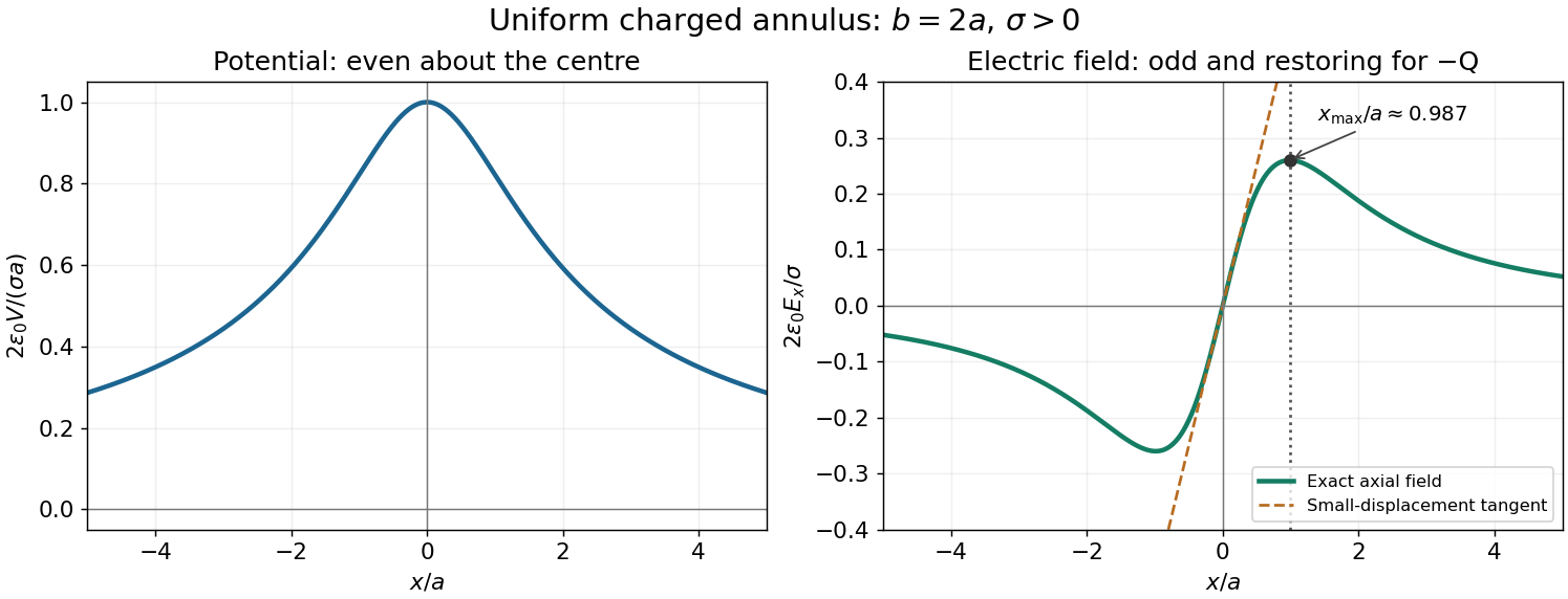
Axial potential and electric field of a uniformly charged annulus
. Original dimensionless curves for and positive surface charge density. The dotted line marks the calculated positive-side maximum of the electric field; the dashed tangent shows its linear behaviour near the centre. Details. Past exam of the physics 2 paper of the University of Oxford 2017 resit 7 a Solution by Codex 0 2026-10-25
Codex 0 2026-10-25The integral and differential forms of Gauss's law in electrostatics areHere is a closed surface bounding a volume , is its outward area vector, is the electric field, is total volume charge density, and is enclosed electric charge. The divergence theorem converts one form to the other. For ideal sheets or point charges, interpret the differential equation with their distributional charge densities.
Past exam of the physics 2 paper of the University of Oxford 2017 resit 2 b Solution by Codex 0 2026-10-25
Codex 0 2026-10-25For the uniform space charge in a grounded spherical cavity, grounding sets the metal's electric potential to zero. With no external sources and zero electric potential at infinity, the exterior electric potential is also zero by the uniqueness theorem for the electrostatic potential. The original shell electric charge is no longer fixed: electric charge can flow to or from earth.
Inside the cavity, Gauss's law gives . Integrating the electric field inward from the zero boundary electric potential givesThe inner surface carries , where , and the outer surface carries zero net electric charge. Only the cavity contributes to the final electrostatic energy:The same result follows from ; the conductor's surface charge contributes zero because its electric potential is zero. This is the final stored electrostatic energy, not the change from the earlier central-charge configuration, whose ideal point charge has divergent self-energy.
Past exam of the physics 2 paper of the University of Oxford 2017 resit 2 a Solution by Codex 0 2026-10-25
Codex 0 2026-10-25The central point charge and spherical boundaries give a spherically symmetric charge distribution. A conductor in electrostatic equilibrium has zero electric field within its material. Consequently a spherical Gaussian surface inside the metal encloses zero net electric charge, so the inner surface carries . The shell's prescribed total electric charge then leaves on its outer surface. Gauss's law givesThe electric field is singular at the ideal central point charge. At each charged surface the normal component has distinct one-sided limits, as required by the electrostatic boundary conditions at a conductor. Spherical symmetry makes the outer surface charge density uniform:
Past exam of the physics 2 paper of the University of Oxford 2017 resit 10 d Solution by Codex 0 2026-10-25
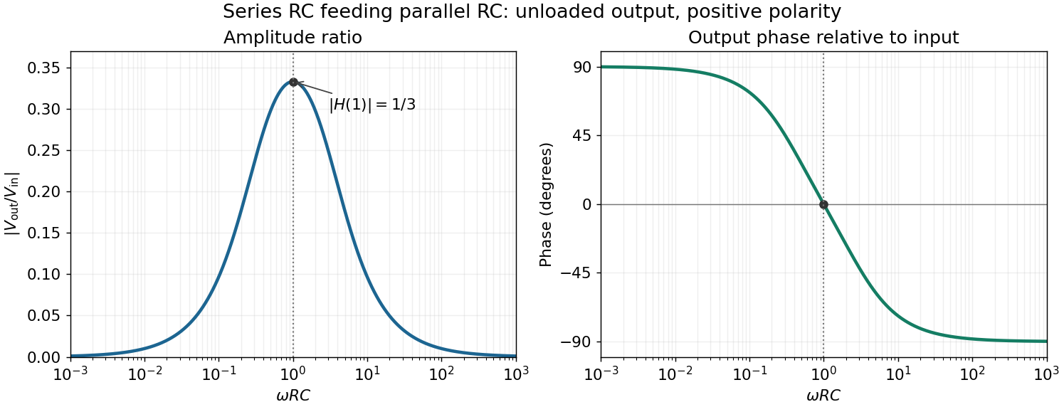
Codex 0 2026-10-25In the chosen phasor convention, output phase minus input phase isThe real part of the denominator is positive, so this principal arctangent is continuous throughout the positive-frequency range. Below , the output leads the input, approaching at low frequency. Above , it lags, approaching at high frequency. At the maximum,The input and output are in phase there, with the positive one-third voltage ratio found above.
Past exam of the physics 2 paper of the University of Oxford 2017 resit 10 c Solution by Codex 0 2026-10-25
Codex 0 2026-10-25For positive angular frequency, the squared amplitude response of the series-parallel RC band-pass filter isIts denominator is minimized exactly when , soThis is a band-pass filter maximum produced entirely by the two RC arms; the drawn electrical circuit contains no inductor. The low- and high-frequency limits areThus the output amplitude tends to zero linearly with at low frequency and as at high frequency. In real time,The upper series capacitor suppresses low frequencies, while the lower shunt capacitor suppresses high frequencies.
Past exam of the physics 2 paper of the University of Oxford 2017 resit 10 b Solution by Codex 0 2026-10-25
Codex 0 2026-10-25The original diagram's upper arm is a series resistor and capacitor; its lower arm is a parallel resistor and capacitor. The output is the upper-minus-lower voltage across that parallel arm. Assume an ideal input voltage source and an unloaded output. Their electrical impedances areFor this series-parallel RC band-pass filter, the voltage divider gives, with ,Taking the real part of yields the steady outputInitial charging contributes decaying transients if the source is switched on at a finite time; the displayed expression is the sinusoidal steady state. The output polarity matters: reversing the indicated output voltage would multiply by .
Past exam of the physics 2 paper of the University of Oxford 2017 resit 10 a Solution by Codex 0 2026-10-25
Codex 0 2026-10-25Use phasors with time dependence . The electrical impedance is the complex number relating the sinusoidal voltage and electric current: is their amplitude ratio and is the voltage phase relative to the electric current. The component laws giveThus the resistor has zero relative phase, the capacitor voltage lags its electric current by , and the inductor voltage leads its electric current by . The ideal capacitor and inductor store and return energy; the real electrical impedance of the resistor describes dissipation.
Past exam of the physics 2 paper of the University of Oxford 2016 9 d Solution by Codex 0 2026-10-25
Codex 0 2026-10-25The largest field in each gap lies at that gap's smaller radius. Thus the quantity to minimize isFor positive , projecting any outside back to that interval reduces both absolute potential drops, so the optimum lies inside it. Within the interval, one candidate maximum decreases linearly with and the other increases linearly. Their maximum is minimized at their intersection, not by making the potential drops equal.
With , , and , the two maxima are and in . Equating them givesThe maximum is halved relative to the two-sphere system and is attained at both and . At and the optimized field is only about ; at the charged middle shell produces a jump.
For plotting, the two-sphere electric potential is . In the three-sphere system it isThe electric potential remains continuous at , while its radial derivative changes there. The graphs show both the continuous potentials and the one-sided gap fields; the marked endpoints identify all maxima.
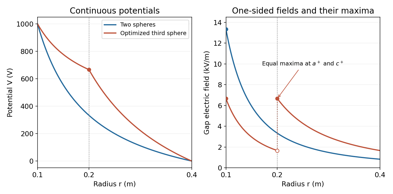
Potential and electric field before and after optimized intermediate-sphere bias
. Details. Past exam of the physics 2 paper of the University of Oxford 2016 9 c Solution by Codex 0 2026-10-25
Codex 0 2026-10-25Inserting an independently biased conducting sphere makes two vacuum gaps, each with its own constant radial electric flux. Let and be the coefficients of . The two potential drops areThereforeThe middle conductor can carry net electric charge, so and need not be equal. Its charge is , consistent with the jump in the normal electric field. For both fields point outwards; outside that interval one of the gap fields reverses direction.
Past exam of the physics 2 paper of the University of Oxford 2016 9 b Solution by Codex 0 2026-10-25
Codex 0 2026-10-25The electric field magnitude falls as throughout the vacuum gap, so its maximum occurs just outside the inner sphere:ThusInside the metal the electric field is zero. The one-sided gap value is the relevant value for dielectric breakdown; the ideal zero-thickness conducting boundary itself should not be assigned a single field value across its surface-charge discontinuity.
Past exam of the physics 2 paper of the University of Oxford 2016 9 a Solution by Codex 0 2026-10-25
Codex 0 2026-10-25Spherical symmetry and the vacuum Gauss's law imply in the gap, where is constant. Integrating the electric field between the two equipotentials givesConsequentlyThe inner charge is , which reproduces the spherical capacitor capacitance . The radial direction is outward for positive and inward for negative ; the formula represents the signed field, not just its magnitude.
Past exam of the physics 2 paper of the University of Oxford 2016 8 d Solution by Codex 0 2026-10-25
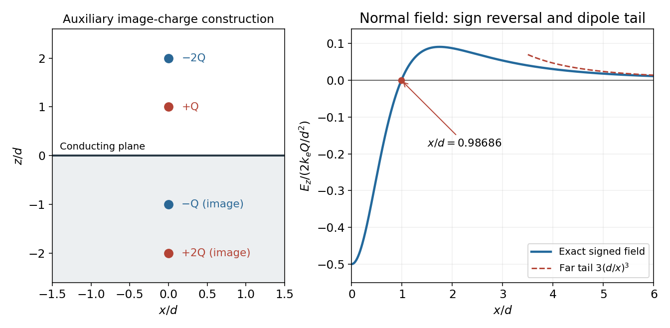
Codex 0 2026-10-25Set the normal electric field to zero and cancel its nonzero overall factor:Taking the power gives , henceThe numerical value is independent of the nonzero magnitude of . Beyond this radius the signed normal electric field is positive. Thus its magnitude first falls to zero, rises again and eventually decays; it is not globally monotone.
For , expanding each denominator givesThis is a dipole rather than a monopole tail. The real-plus-image charge distribution has zero total charge and dipole moment ; in its equatorial plane a dipole produces , confirming the coefficient and sign.
Past exam of the physics 2 paper of the University of Oxford 2016 8 c Solution by Codex 0 2026-10-25
Codex 0 2026-10-25Let denote the radial distance from the axis in the plane, and write . A charge at height and its image give a combined normal electric field at ; the tangential components cancel. Superposing the two pairs yieldsThe conductor boundary condition gives , soTo integrate the induced surface charge, use concentric annuli of area . Since ,The local surface charge density is negative near the origin but positive farther out; integrating only the negative patch would miss the total. The total real charge is , so the induced also agrees with the sum of the two image charges. An isolated finite plate constrained to zero net charge would require a different global boundary-value problem; the formula is the infinite-plane solution just specified.
Past exam of the physics 2 paper of the University of Oxford 2016 8 b Solution by Codex 0 2026-10-25
Codex 0 2026-10-25Use the standard infinite-plane boundary condition: the sheet is an equipotential, with no imposed uniform background electric field and the electric potential tending to zero far from the localized charges. The images of at and at are at and at .
At the point directly below the real charges, horizontal components vanish. The first real-image pair contributes along , while the second contributes . ThereforeFor , the electric field points downwards into the sheet. The expression is the one-sided vacuum limit; the electric field inside the conducting material is zero. A prescribed uniform background field would be an additional boundary condition and would change this result.
Past exam of the physics 2 paper of the University of Oxford 2016 8 a Solution by Codex 0 2026-10-25
Codex 0 2026-10-25The method of images replaces a conducting boundary by fictitious point charges placed outside the physical region being solved. Choose their positions and strengths so that the resulting electric potential has the required constant value on each conductor. The uniqueness theorem for the electrostatic potential then guarantees that this solution equals the physical solution in the allowed region, provided the other boundary conditions are also satisfied.
For a plane held at zero electric potential, a real charge a height above the plane has an image the same distance below it. The pair's electric potential vanishes everywhere on the plane. Its tangential electric field consequently vanishes there, as required in electrostatic equilibrium. The image is a mathematical representation of the induced surface charge, not a physical charge placed inside the conductor. Forces on the real charge can be computed from the image field, but total physical electrostatic energy must account for the conductor's induced response rather than simply counting a full real-plus-image pair energy.
Past exam of the physics 2 paper of the University of Oxford 2016 7 b Solution by Codex 0 2026-10-25
Codex 0 2026-10-25Interchange the input and feedback components: put the capacitor between the input and the inverting terminal, and the resistor between the output and the inverting terminal. Keep the non-inverting terminal grounded, as in the lower circuit above. For an ideal operational amplifier under unsaturated negative feedback, the inverting node remains at virtual ground.
The input capacitor current is . It flows through the feedback resistor, givingThis is an inverting op amp differentiator. Its ideal gain magnitude increases with frequency, so it strongly amplifies high-frequency noise. Practical differentiators include components that restrict the useful band and stabilize feedback; that qualification does not change the displayed ideal low-amplitude relation within the operating band.
Past exam of the physics 2 paper of the University of Oxford 2016 7 a Solution by Codex 0 2026-10-25
Codex 0 2026-10-25Use an ideal operational amplifier with its non-inverting terminal grounded, an input resistor and a feedback capacitor , as in the upper circuit. Stable unsaturated negative feedback holds the inverting terminal at virtual ground, while the input current into the amplifier itself vanishes.
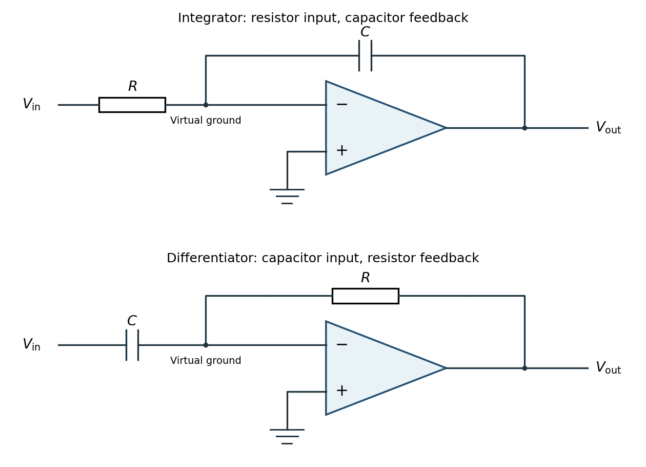
Inverting operational-amplifier integrator and differentiator circuits
. Details. Applying Kirchhoff's current law at the inverting node givesThus the circuit is an inverting op amp integrator, with its integration constant set by the initial capacitor charge. A constant input makes the output ramp until a real amplifier reaches a supply rail. A practical low-frequency design usually adds a large feedback resistor to limit drift; the ideal integral relation applies where the feedback capacitor dominates.
Pinned article: Introduction to the OurBigBook Project
Welcome to the OurBigBook Project! Our goal is to create the perfect publishing platform for STEM subjects, and get university-level students to write the best free STEM tutorials ever.
Everyone is welcome to create an account and play with the site: ourbigbook.com/go/register. We belive that students themselves can write amazing tutorials, but teachers are welcome too. You can write about anything you want, it doesn't have to be STEM or even educational. Silly test content is very welcome and you won't be penalized in any way. Just keep it legal!
Intro to OurBigBook
. Source. We have two killer features:
- topics: topics group articles by different users with the same title, e.g. here is the topic for the "Fundamental Theorem of Calculus" ourbigbook.com/go/topic/fundamental-theorem-of-calculusArticles of different users are sorted by upvote within each article page. This feature is a bit like:
- a Wikipedia where each user can have their own version of each article
- a Q&A website like Stack Overflow, where multiple people can give their views on a given topic, and the best ones are sorted by upvote. Except you don't need to wait for someone to ask first, and any topic goes, no matter how narrow or broad
This feature makes it possible for readers to find better explanations of any topic created by other writers. And it allows writers to create an explanation in a place that readers might actually find it.
Figure 1. Screenshot of the "Derivative" topic page. View it live at: ourbigbook.com/go/topic/derivativeVideo 2. OurBigBook Web topics demo. Source. - local editing: you can store all your personal knowledge base content locally in a plaintext markup format that can be edited locally and published either:This way you can be sure that even if OurBigBook.com were to go down one day (which we have no plans to do as it is quite cheap to host!), your content will still be perfectly readable as a static site.
- to OurBigBook.com to get awesome multi-user features like topics and likes
- as HTML files to a static website, which you can host yourself for free on many external providers like GitHub Pages, and remain in full control

Figure 2. You can publish local OurBigBook lightweight markup files to either OurBigBook.com or as a static website.
Figure 3. Visual Studio Code extension installation.
Figure 5. . You can also edit articles on the Web editor without installing anything locally. Video 3. Edit locally and publish demo. Source. This shows editing OurBigBook Markup and publishing it using the Visual Studio Code extension. 
- Infinitely deep tables of contents:




All our software is open source and hosted at: github.com/ourbigbook/ourbigbook
Further documentation can be found at: docs.ourbigbook.com
Feel free to reach our to us for any help or suggestions: docs.ourbigbook.com/#contact